In this post, you will learn how to implement pivot charts in your Excel spreadsheets and understand how they are linked to pivot tables.
What are Pivot Charts?
Pivot Charts are interactive graphical representations of a dataset in a pivot table. The Pivot Chart Filter Pane appears when you create a PivotChart and it is used to sort and filter the PivotChart’s dataset. They display categories such as data markers, data series, and axes similar to standard charts.
How to Create a Pivot Chart in Excel?
You can create a pivot chart by using two ways.
- Creating Pivot Charts from Scratch
- Create a Pivot Chart from Existing Pivot Table
Creating Pivot Charts from Scratch
Creating a pivot chart from scratch is as simple as creating a pivot table.
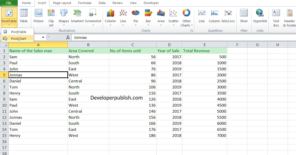
- Click on the required cells in your dataset and from the Insert tab under the tables group click on the drop-down arrow in the Pivot Table option.
- From the drop-down menu, click pivot chart.
- The Create PivotTable with PivotChart dialog ox pops and it default selects the data range ( You can change the data range here) and choose the location for the chart.
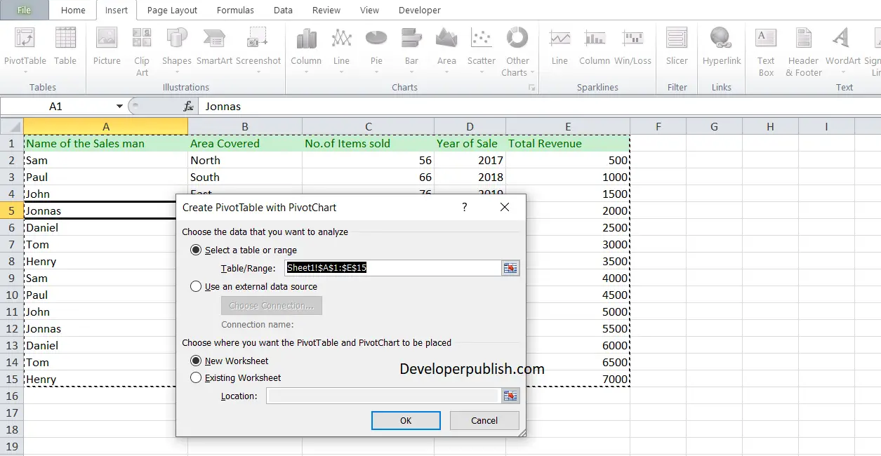
- Click OK.
- Now, you can see a blank pivot table and pivot chart in a new worksheet.
Note: When you insert a pivot chart, the pivot table is automatically inserted. And, if you just want to add a pivot chart, you can add your data into Power Pivot Data Model.
- In pivot chart Layout Labels, there are four components like we have in a pivot table.
- Axis: Axis in the pivot chart is similar to rows in our pivot table.
- Legend: Legend in pivot chart is similar to columns in our pivot table.
- Values: We are using quantity as values.
- Report Filter: You can use a report filter to filter your pivot chart.
Create a Pivot Chart from Existing Pivot Table
If you already have a pivot table in your worksheet then you can create a pivot chart to that by using the below steps.
- Click any of the cells from your pivot table.
- From the Insert tab in the ribbon, under the Charts group, click Pivot Chart and select the chart which you want to use.
- Click Ok.
New pivot chart will be inserted in the same worksheet where you have your pivot table.
Note: You can use the shortcut key for a quick access. Just select the cells in your pivot table and press F11 to insert a pivot chart.