Report Layout in Excel Pivot Table

In this post, you’ll learn about Report Layout in Excel Pivot Table and how to use it in your Excel spreadsheet.             

Report Layout in Excel Pivot Table

Excel has a super cool feature where you can design and layout format of a Pivot Table. When you want to enhance the report layout so that you can alter format to make the data look easier to read and scan for details.

The following modifications can be done to the PivotTable. You can alter the form and the way that fields, columns, rows, subtotals, empty cells and lines are displayed.

Excel has a set of predefined styles, banded rows, and conditional formatting that you can apply on the Pivot Table.

Change the layout form of a PivotTable

You can choose from the following three forms.

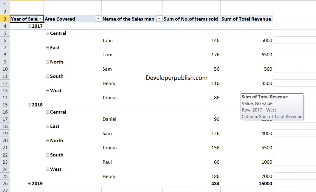
Compact form 

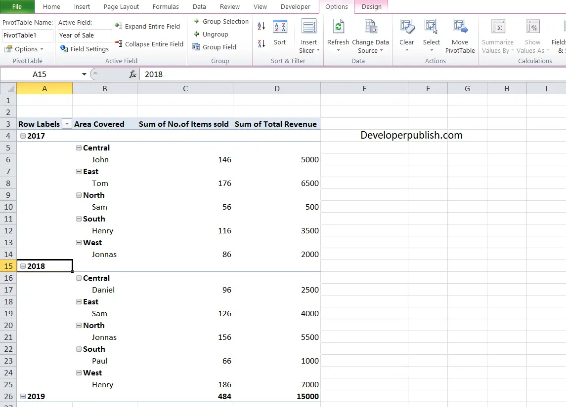
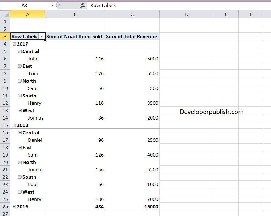
It is the common way of presenting a data in a pivot table. Let’s say it is the default layout when we insert fields in a Pivot table.

The compact form displays data from different row fields in one column and uses indentation to distinguish between the items from different fields.

Expand and Collapse buttons are enabled to display or hide details in compact form. It is more readable than other layout forms, which makes it the most desired form layout.

Tabular form   

The tabular form displays each row field in a separate column and it also has space for field headers.

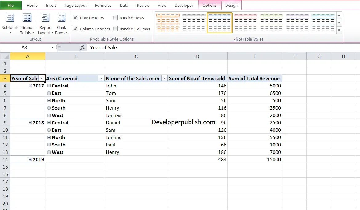
Outline form

This is pretty much similar to tabular form with an additional advantage that it automatically displays subtotals at the top of every group.

How to Change the PivotTable to compact, outline, or tabular form?

To Change the layout form of a PivotTable:

• Click anywhere in the PivotTable.
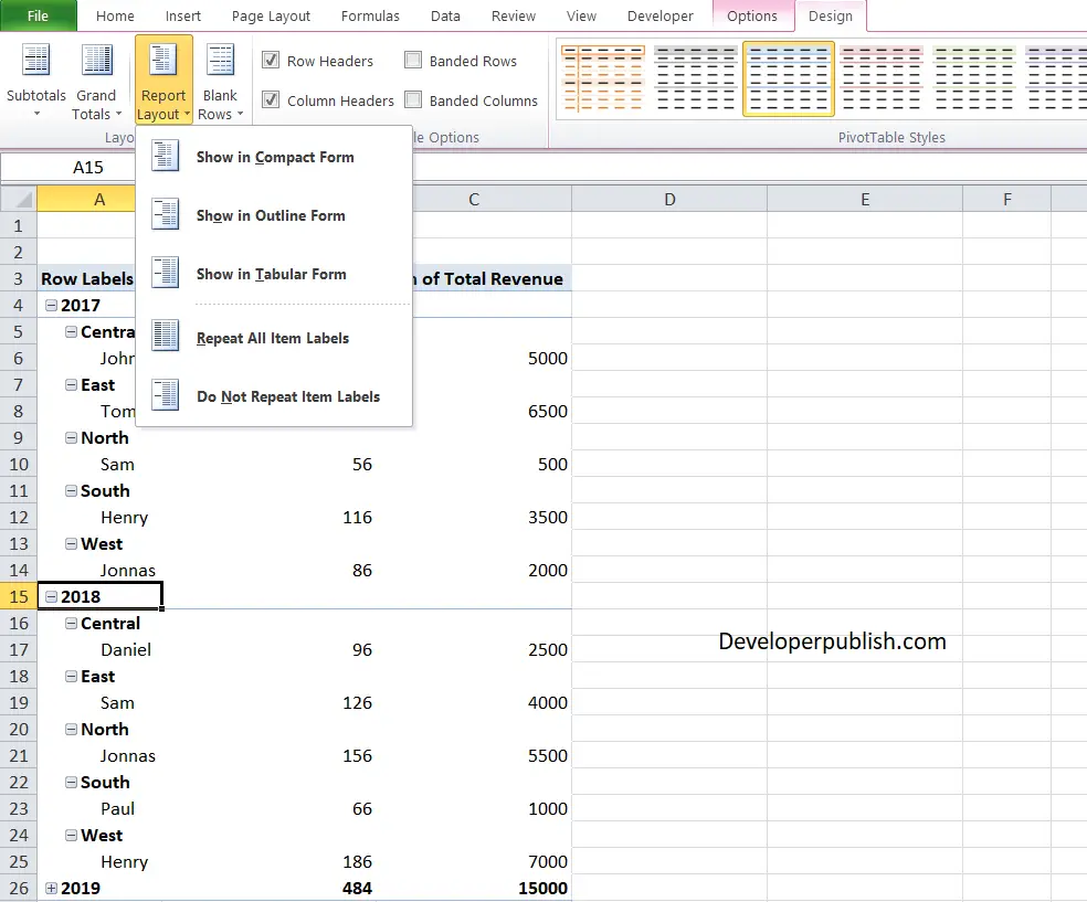
• Under the Design tab in the ribbon, you can find the Report layout option or icon in the Layout group.
• Click on the Report Layout option, and from the drop-down choose any one of the options:
  1. Compact Form.
  2. Show in Outline Form.
  3. Show in Tabular Form.

Change the way item labels are displayed in a layout form

To Change the way item labels are displayed in a layout form:

• Select a row in the pivot table.
• Under the Options tab, in the Active Field group, click Field Settings.
• The Field Settings dialog box opens, under the Layout & Print tab, from the Layout section, choose your desired style.

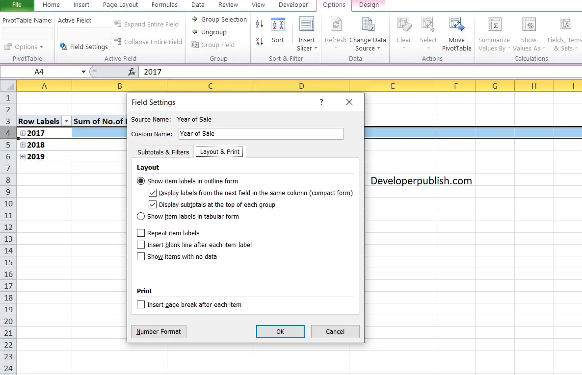
• Show item labels in outline form.
  1. Display Labels from the next field in the same column (compact form).
  2. Show item labels in tabular form.

To display or hide labels from the next field in the same column in compact form, check or uncheck the option in the dialog box.