In this post, you’ll learn about the GETPIVOTDATA Function, its syntax and the way of using the GETPIVOTDATA Function in an excel spreadsheet.
What is GETPIVOTDATA Function?
The GETPIVOTDATA Function is a Lookup and Reference function. The GETPIVOTDATA Function calculates specific data from pivot data and returns visible data from a Pivot Table by name based on structure, instead of cell reference.
In financial analysis, the Pivot table is useful to facilitating deeper analysis of given data.
Syntax
=GETPIVOTDATA(data_field, pivot_table, [field 1, item 1],..)
Arguments:
- = – built-in function.
- GETPIVOTDATA() –function name.
- data_field – the name of the Pivot Table field which contains data for retrieval. It must be within double quotes.
- pivot_table – a reference to any range of cells in a pivot table, to determine the retrieval of data.
- field 1, item 1,.. – (optional) it can be up to 1 to 26 pairs of names and items which you want to retrieve the data. It acts like filters, which limits data retrieval based on the structure.
GETPIVOTDATA Function will continuously and correctly work even when the pivot table change, still the field reference is present.
Note:
- GETPIVOTDATA Function is automatically generated when a reference cell in a pivot table is pointed by selecting. You can also type the address of the cell to be calculated(instead of clicking).
- To disable the feature entirely “Generate GETPIVOTDATA” in the menu at Pivot Table Tools > Options >Uncheck the Generate GETPIVOTDATA option.
- #REF! Error – if the field is given incorrectly.
- #REF! Error – if reference to pivot_table is invalid.
Remember;
- Fields and items must be in pairs and also given as text values.
- Based on Date data’s, use Excel’s native format or as function names Data Function.
- Based on Time data, it must be given as decimal or as Time Function.
How to use GETPIVOTDATA Function in Excel?
GETPIVOTDATA Function calculates the PIVOT Data and gives visible value of given data .
Example:
Step 1:
Open the workbook in your Microsoft Excel.
Step 2:
Enter the data, in the workbook.
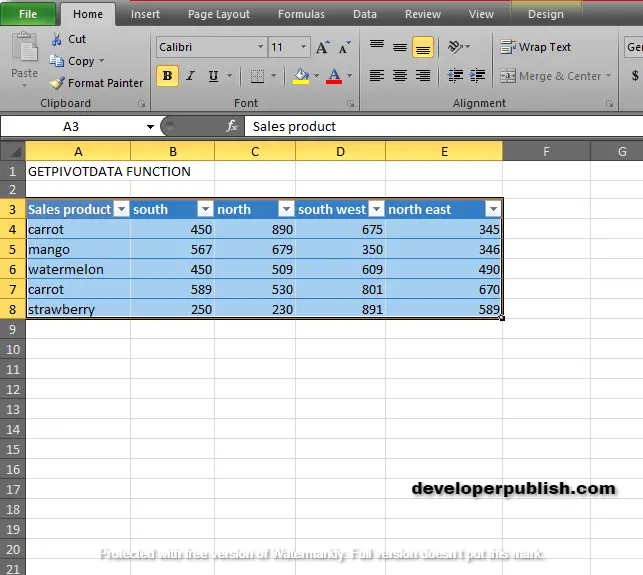
In this example, we created a pivot table with sales product and the sales amount according to the directions.
STEP 3:
In the new cell, give the syntax. Start with ‘ =’ for every functions, GETPIVOTDATA Function to initiate functions name, followed by open parenthesis or just give = sign and then select the value in the pivot table.
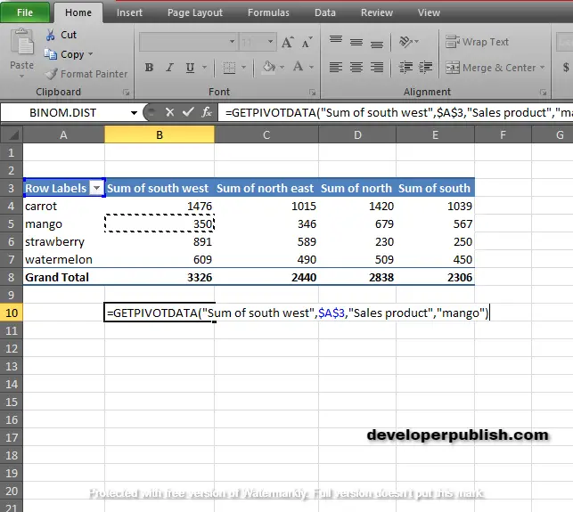
According to the example, the argument of the syntax is data_field is sum of south west, pivot_table is $A$3, field 1 is sales product and item 1 is mango.
STEP 4:
Press enter to get the GETPIVOTDATA value.
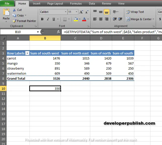
It return the visible pivot value.
CREATING PIVOT TABLE;
- Select the data > click PIVOT Table from the insert tab.
- Then a dialogue box appears.
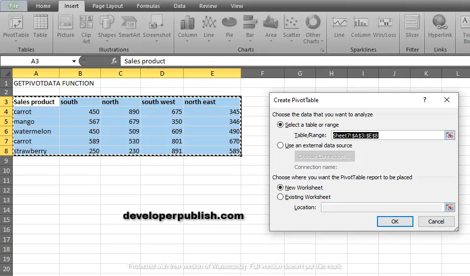
Click ok .
3. Now the PIVOT table dialogue box appears. Choose the fields to add to the report.
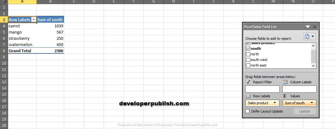
Select the box, now move the south, north, south-west, northeast by clicking and dragging to the value section.
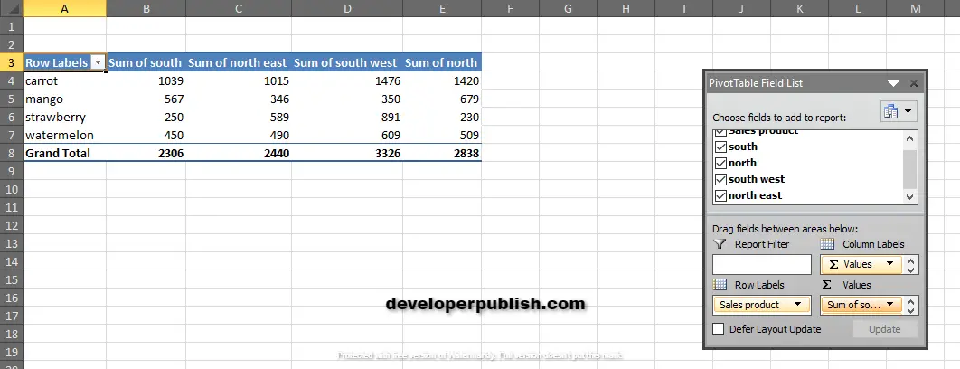
Now the pivot table is ready to calculate with the total.