RANDBETWEEN Function in Excel
In this post, you will learn about the RANDBETWEEN Function in Excel, how to use in your excel spreadsheets.
Syntax
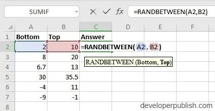
=RANDBETWEEN(bottom, top)
The syntax has two arguments
- bottom – This argument holds the first number, which is the lower value of the range
- top – This argument holds the second number, which is the upper value of the range.
How to use RANDBETWEEN in Excel?
- The function returns a random number between the range of the given two numbers. And the value changes as the function revaluates each time the spreadsheet is calculated or opened.
- To start with entering the numbers in an excel sheet, and in a new cell enter the syntax of the function. Highlight the numbers to include them in the function.
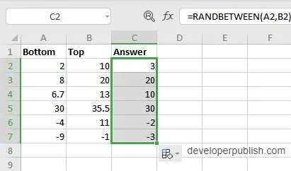
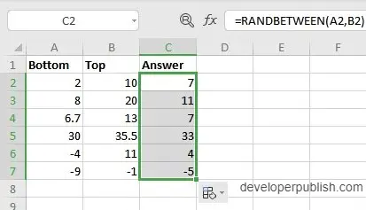
- Press enter to display the answer and use the fill handle to apply the function in the rest of the data.
- The below example uses the same values for the arguments, but when recalculated gives different answers.
Additional Points:
- The syntax accepts positive, negative, and decimal numbers.
- The function returns a different value after each recalulation of the syntax.
- Note that the bottom argument value has to be less than the top argument value, or the function will return #NUM! error.
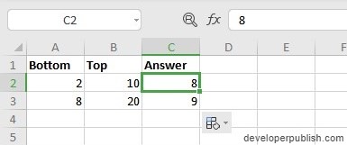
- To keep the answer constant, select an empty cell and enter the syntax in the formula bar. Press f9, this performs the function once, giving a static result.
- When the answer is seen displayed in the formula tab, this means the answer is static.


Leave a Review