In this post, you will learn about a Matrix function – MINVERSE function in Excel, how to use it in your excel spreadsheets.
MINVERSE Function in Excel
The function returns the inverse matrix of the given array.
Note:
- Array – An arrangement of objects in rows and columns.
- Matrix – An array of many numbers.
Syntax
=MINVERSE(array)The syntax has a single argument
- array – This holds the data of the square matrix.
How to use MINVERSE Function in Excel?
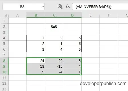
- The function returns the inverse matrix of the given array.
- It is important to note that the array has to be a square matrix, or else the syntax returns #VALUE!.
- Note: A square matrix is a combination of equal numbers of columns and rows.
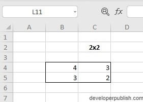
Start with a Square Matrix in the Excel sheet.
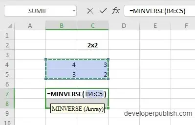
- Highlight the new cells in a similar structure as the matrix and enter the syntax.
- Highlight the matrix to include it in the syntax.
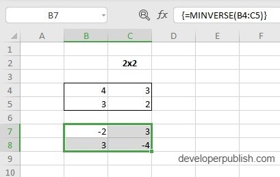
To display the answer press Ctrl + Shift +Enter, this will display the answer in a complete matrix form. Or else only one value of the matrix will be displayed.
Additional Points:
- The function accepts negative numbers and decimal numbers.
- When non – numeric values and alphabets are used the syntax returns the #VALUE!.
- Empty cells in the source array will cause the function to return #VALUE!.
- The MINVERSE Function with Ctrl + Shift +Enter step, is called a multi – cell array formula.


