In this post, you’ll learn about summarizing Pivot table data in your Microsoft Excel spreadsheet.
Summarizing Pivot Table Data in Excel
Excel offers you a variety of methods to summarize your data in the Pivot table. Some of its summarize functions are Sum, Count, and Average.
Whenever you place a field in the ∑ Values in the field list pane, it automatically sums the value in the column. The default function for the numeric value fields in the PivotTable is the Sum function, but you can choose a different summary function.
- In the PivotTable, right-click the Grand Total field, and then click Summarize Values By.
- From the drop-down menu, click on the function that is necessary.
Summary options and its Functions
Here is the list of summarize options available along with its function.
| Summary Options | Functions |
| Sum | The normal addition function. It sums up the values present in the column. It’s the default function for value fields that have numeric values. When the sum function is applied and any blank or non-numeric values are changed to 0 in the PivotTable so they can be summed. |
| Count | It displays the number of nonempty values. It is used by default for value fields that have non-numeric values or blanks. |
| Average | Displays the average of the given values. |
| Max | Displays the largest value. |
| Min | Displays the smallest value. |
| Product | Displays the product of the values. |
| StDev | An estimate of the standard deviation of a population, where the sample is a subset of the entire population. |
| StDevp | The standard deviation of a population, where the population is all of the data to be summarized. |
| Var | It displays the estimate of the variance of a population, where the sample is a subset of the entire population. |
| Varp | It displays the variance of a population, where the population is all of the data to be summarized. |
| Distinct Count | It displays the number of unique values. This summary function only works when you use the Data Model in Excel. |
Let’s see the summarize functions with an example.
Take a look at the following Pivot table.
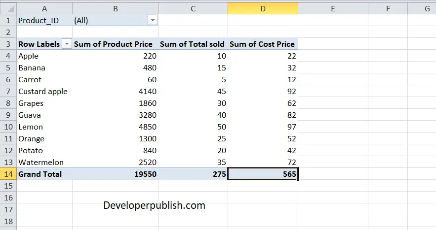
- In the Grand Total value of Sum of cost price column, right-click and click on the “summarize value by” option
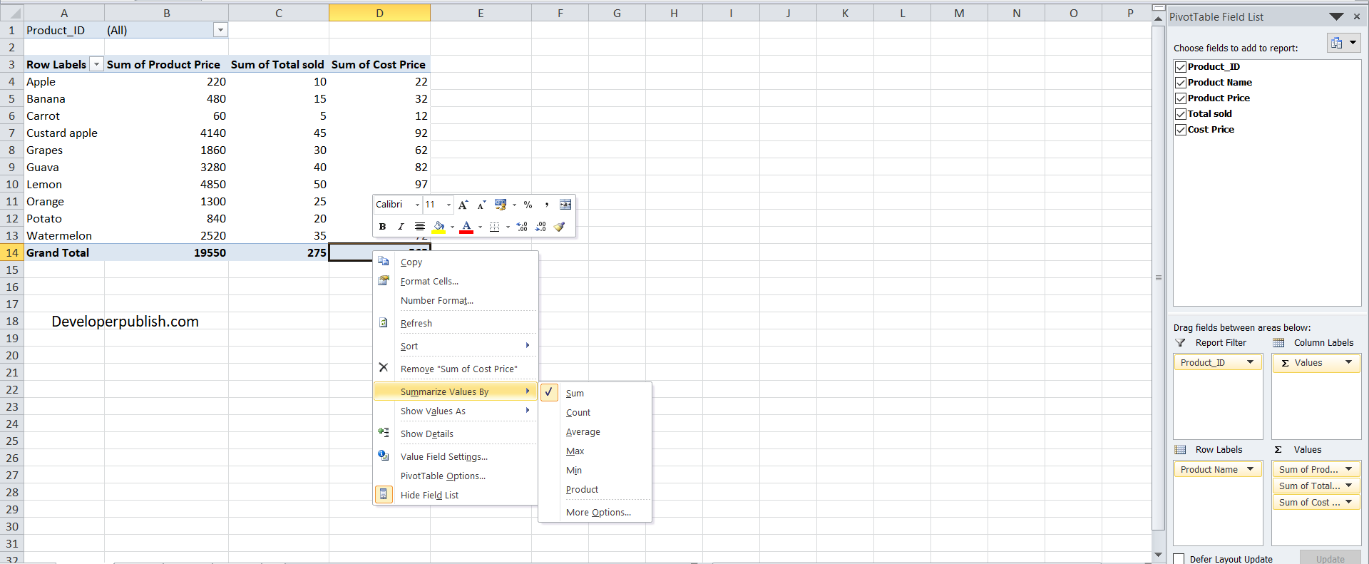
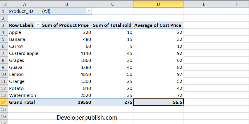
- In the drop-down menu, choose the average value option.

- The table immediately displays the average cost price of the products.
- If you choose the “Max” option, it displays the maximum value present in the column.
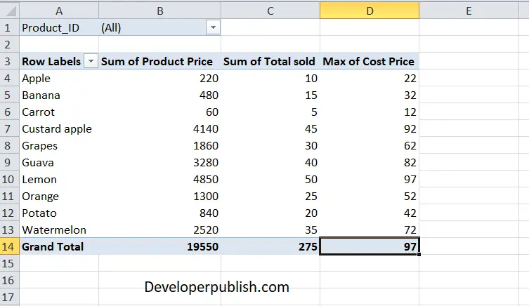
You can repeat the steps for other options too.


