In this post, you’ll learn about DEVSQ Function, its syntax and the way of using DEVSQ Function in Excel spreadsheet.
What is DEVSQ Function?
The DEVSQ Function is a statistical function. The DEVSQ Function in Excel calculates and returns the sum of squared deviation from the mean of given set of data without dividing N or N-1.
In financial analysis, DEVSQ Function is very important in understanding the variance of daily stock values which signifies market instability and the risks of investors.
Syntax
=DEVSQ(number 1, [number 2],..)
Arguments:
- = – built-in function.
- DEVSQ() – function name.
- number 1 – first value.
- Number 2 – (optional) additional values. The arguments can be up to 1 to 255 in MS Excel 2007 and also in later versions but in 2003 and earlier version there can be only 30 arguments.
Variance and Standard deviation function deals with negative deviations by squaring the deviations before the average.
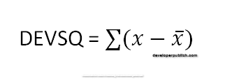
The Equation for sum of squared deviations is:
Notes:
- Arguments can be numbers, names, array, zero or reference that contains numbers.
- Ignores empty cells, logical values and text.
- You can also use single array or reference instead of arguments.
- #VALUE! Error – when number or text given directly to DEVSQ Function.
- #NUM! Error – text values are given as a value.
How to use the DEVSQ Function in Excel?
DEVSQ Function is used to calculate the sum of squared deviations.
Example:
Step 1: Open the workbook in your Microsoft Excel.
Step 2: Enter the data, in the workbook.
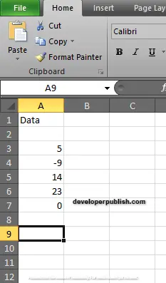
In this example, we gave some random values such as numeric values including negative number and a zero to calculate DEVSQ Function.
STEP 3:
In the new cell, give the formula or the syntax. Start with ‘ =’ for every functions, DEVSQ to initiate functions name, followed by open parenthesis.
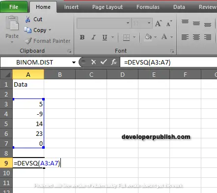
The given data is in the cell reference A3 to A7.
STEP 4:
Press enter to get the result.
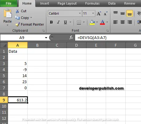
The result for the given data is 613.2.


