How to insert drop down list in Microsoft Excel 2016 ?
If you are one of the users who use excel more frequently at work, for instance, Data Analytics user, you would have come across the requirement to insert a drop-down list in excel more regularly. In this article, we will look at how to do that in a step by step manner.
In this article, we will look at how to do that in a step by step manner.
Although this post talks about inserting a drop-down list in Excel 2016, this excel tip is applicable for other versions. If you are using Microsoft Excel 2013, Microsoft Excel 2016, and Microsoft Excel 2019, it would also work fine.
How to insert drop-down list in Microsoft Excel 2016 ?
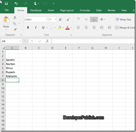
1. Firstly, Open your excel workbook in Microsoft Excel 2016 and then create a list of data that you want to insert in the drop-down list. In this example, let’s have the sheet2’s cell A3 to A7 contain the list items.
Select the range of cells where you want to display the drop-down list. In this example, let’s select the cell D3.
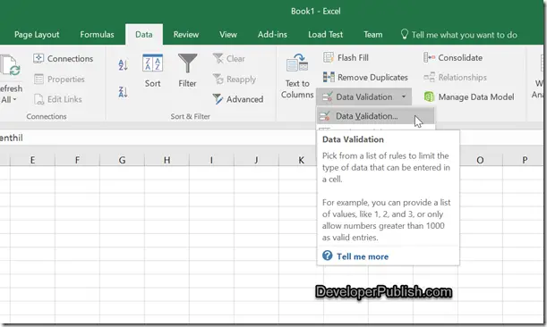
3. After that, click the “Data Tab” and select Data Validation –> Data Validation.
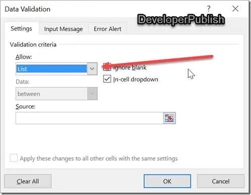
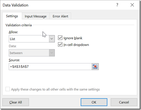
4. In the Data Validation dialog, select “List” in the “Allow” dropdown list in the Settings tab.
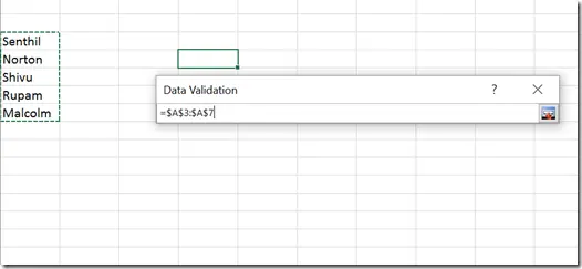
5. Click the symbol in the DataValidation tab to select the source cells’ range to fill the drop-down list data. In our example, we should choose “A3 to A7” and press the enter key.
6. You should see the following in the Data Validation dialog.
7. Finally, click the OK button in the Data Validation Tab, and you should see the drop-down list inserted in the cell D3 with the required data.




Leave a Review