In this post, you will be guided through simple and easy-to-follow steps to use the CUMPRINC function in Excel.
Microsoft Office Excel provides the CUMPRINC function, which helps to return the cumulative principal paid on a loan between a start period and an end period. In other words, CUMPRINC is used to calculate and verify the total principal paid on a loan, or the principal paid between any two payment periods.
CUMPRINC Function in Excel
The CUMPRINC Function returns the returns the cumulative principal paid on a loan between start_period and end_period. It is used to calculates the cumulative payment on the principal of a loan or investment, between two specified time periods. It is a built – in Excel function categorized under Financial Functions.
CUMPRINC Syntax
=CUMPRINC(rate, nper, pv, start_period, end_period, type)
CUMPRINC arguments and functions
- rate (required) – The interest rate per period.
- nper (required) – The total number of payments for the loan.
- pv (required) – The present value, or total value of all payments now.
- start_period (required) – First payment in calculation.
- end_period (required) – Last payment in calculation.
- type (required) – When payments are due. 0 = end of period. 1 = beginning of period.
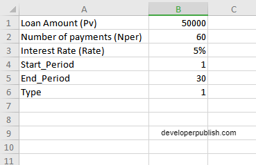
Consider an example of a loan amount of $50,000 where the interest is paid at a rate of 5% monthly with a total of 60 payments. Here, we consider the start period will be 1, the end period will be 30, and the type, that is the time for the loan is considered as 1.
How to use the CUMPRINC function in Excel?
- Open Microsoft excel and launch a workbook or create a new Excel sheet.
- As said in the description, you need the values of all the above arguments to carry out the CUMPRINC function and get the correct and desired cumulative principal.
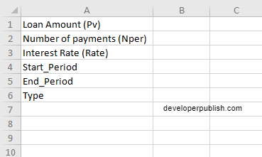
- Enter the arguments in the same order of the syntax, one below the other, as shown in the picture below.
- At this time, in a similar way enter the values of each of the arguments in their corresponding adjacent cells in the worksheet.
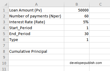
- Below the tabulated list of arguments, select a cell and enter “Cumulative Principal”, the cell to the right will display the value of the formula (making identification easier).
- When entering the formula, always start with the “=” operator. After entering the “=” operator enter CUMPRINC to initiate the formula followed by an open parenthesis. Excel recognizes “=’ as the start of a formula, if not included, excel will not accept and evade the execution of the function.
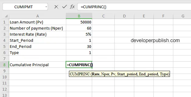
- With the parenthesis open, select the arguments in the order of syntax. The position of the cell will be visible in the formula. According to the order of the syntax, the value of the argument must be selected followed by a comma. The change in color of the cells aids to identify the name and of the cells in the formula.
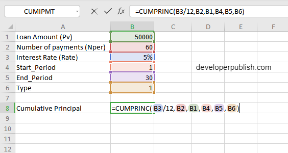
- For the rate argument of the syntax, most of the interest rates are given annually, but here since it is a cumulative function, we are calculating for each month, that is 12 months in total, therefore the rate percent should be divided with 12.
- For the type argument, there are only 2 options to enter, that is 0 or 1. Enter 1 if the payment is made at the beginning of the period or enter 0 if the payment is paid at the end of the period
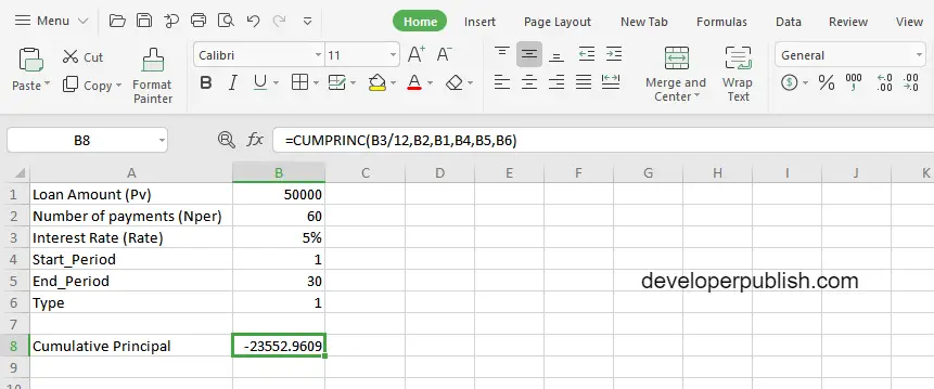
- To conclude, close the parentheses and click enter. The cell which contains the formula will display the cumulative principal.

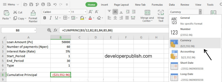
- Change the value from the numerical to currency, by using the option under the home tab.
Note
- As the interest is quoted as an annual interest rate, for this loan we will make a payment every month, which is 12 payments in a year. So we have to convert the rate and the number of payments from annually to monthly depending on the data.
- For the interest rate, we should divide it by 12 to get the monthly interest rate. For the total number of payments, in the given example, it is 60, which is already quoted as monthly, that is 5*12 = 60


