In this post, you will be guided through simple and easy-to-follow steps on how to use the AMORLINC function in Excel.
Microsoft Office Excel provides the AMORLINC function, which helps the users to calculate the depreciation value of an asset for a particular accounting period. This is a built-in function under the category Financial Function in Excel.
AMORLINC Function in Excel
The Excel AMORLINC function returns the depreciation for each accounting period of an asset on a prorated basis.
In simpler terms, the AMORLINC function helps in giving the depreciation value of an asset for a certain period of time. The AMORLINC function syntax is similar to that of the AMORDEGRC function in Excel.
AMORLINC Syntax
AMORLINC(cost, date_purchased, first_period, salvage, period, rate, [basis])
The AMORLINC function and arguments
- Cost (Required) – The cost of the asset.
- Date_purchased (Required) – The date of the purchase of the asset.
- First_period (Required) – The date of the end of the first period.
- Salvage (Required) – The salvage value at the end of the life of the asset.
- Period (Required) – The period.
- Rate (Required) – The rate of depreciation.
- Basis (Optional) – The year basis to be used.
How to use the AMORLINC function in Excel?
1) Open Microsoft excel and launch a workbook or create a new Excel sheet.
2) As said in the description, you need the values of all the above arguments to carry out the AMORLINC function and get the correct and desired depreciation value.
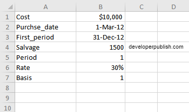
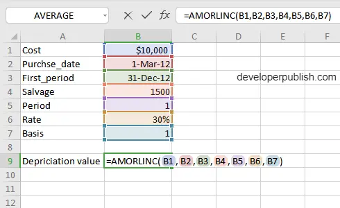
3) Enter the arguments in the same order of the syntax, one below the other, as shown in the picture below.

4) At this time, in a similar way enter the values of each of the arguments in their corresponding adjacent cells in the worksheet.
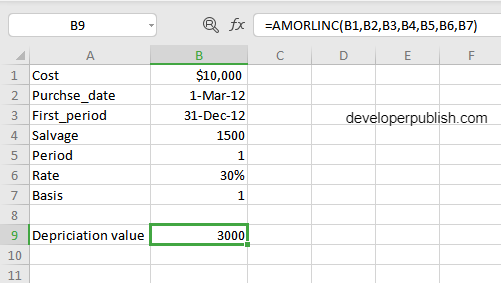
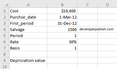
5) Below the tabulated list of arguments, select a cell and enter “Depreciation value”, the cell to the right will display the value of the formula (making identification easier).
6) In addition, bringing to note that when entering the formula, it should always start with the “=” operator. After entering the “=” operator enter AMORLINC to initiate the formula followed by an open parenthesis. Excel recognizes “=’ as the start of a formula, if not included, excel will not accept and evade the execution of the function.
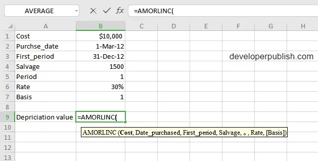
7) With the parenthesis open, select the first argument value. The position of the cell will be visible in the formula. According to the order of the syntax, the value of the argument must be selected followed by a comma. The change in color of the cells aids to identify the name and of the cells in the formula.
8) To conclude, close the parentheses and click enter key. The cell which contains the formula will display the value of depreciation of the asset.