INTERCEPT Function in excel
In this post, you’ll learn about INTERCEPT Function, its syntax and the way of using INTERCEPT Function in an excel spreadsheet.
What is an INTERCEPT Function?
INTERCEPT refers to the point on the axis, in which the line crosses over on it.
INTERCEPT Function is a statistical function. The INTERCEPT Function in Excel calculates and returns the point in which the regressive line interact with the y-axis based on known x and known y value.
Syntax
=INTERCEPT(known_y’s, known_x’s)
Argument:
- = – built-in function.
- INTERCEPT() –function name.
- known_y’s –the known numeric data points(y-value, dependent value).
- known_x’s – the known numeric data points(x-value, independent value).
The INTERCEPT point is based on a fit regressive line, which is plotted through known x and known y value. You can use INTERCEPT Function to calculate the dependent variable, when the independent variable is zero(0).
Notes:
- Arguments can be names, numbers, array, zero or reference that consists of only numbers.
- Ignores logical values, empty cells and text.
- To find x intercept, set y=0 (to solve x).
- To find y intercept, set x=0 (to solve y).
- #DIV/0! – If it contains only one set of point.
- #N/A! – if number of known_y’s is different from known_x’s.
Equation:
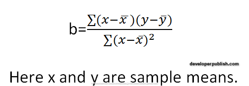
The Equation for regressive line(a) intercept is;

b is a slope. The same formula is also used for the SLOPE Function.
How to use INTERCEPT Function in Excel?
INTERCEPT Function returns the point in which the regressive line interact with known values.
Example:
STEP 1:
Open the workbook in Microsoft Excel.
STEP 2:
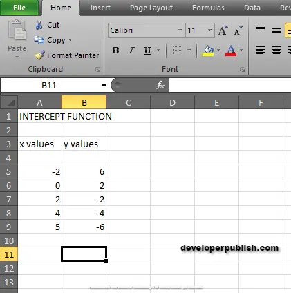
Enter the data in the workbook.
In this example, we just gave some random values as x axis and y axis values.
STEP 3:
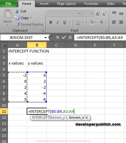
In the new cell, give the formula. First always start with ‘ =’ for every functions, INTERCEPT function name, followed by the open parenthesis, the arguments of the syntax.
According to the arguments, you need to calculate known_y’s. In this example the known_y’s values is from B5 : B9.
STEP 4:
Keep a comma, then the next argument is known_x’s.
The known_x’s is also from A5:A9.
STEP 5:
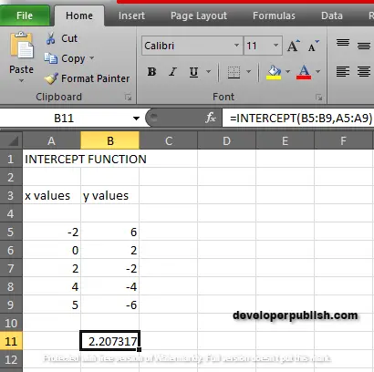
Press enter to get the INTERCEPT values.
Return 2.207317, which is almost 2 to the given data.




Leave a Review