“Filters in Excel” is a way to show the data you need and hide the information you don’t need. There are some ways to handle this Filter, and this post will explain it.
How does Filter in Excel work?
This works on the data that has to be sorted in the basis of the “Greatest One” or the “Top 10”. Now let’s see how does it perform the activity.
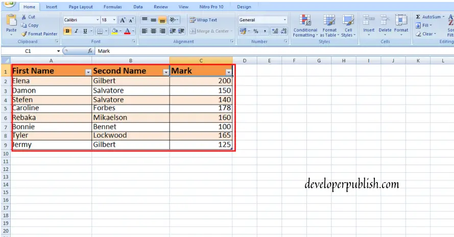
- To filter a particular data, (either it may be numerical data or text) just select a cell & go to the “Data” bar in the ribbon on the top of the excel sheet. There you will see the “Filter” option, click on it.
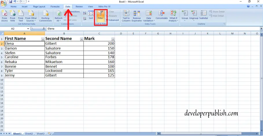
2. Once you select the Filter option, you see that all the coumns’s first cell will have the Header arrow in it.
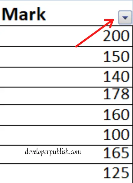
3. Select the Header arrow, then you will get a pop-up with the list of options. You can choose either the text filter or the number of filter from the list of options.
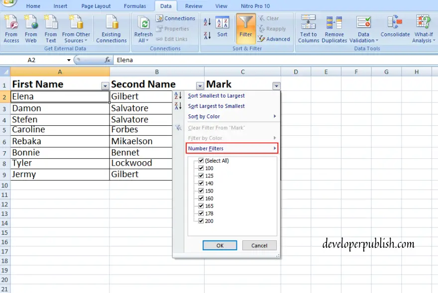
Note: The text filter option will show up if the Data entered are text, else the number of filters will show up for the numerical Data.
4. This Number Filter option gives a list of options to filter the data like greater than or less than, etc. Or you may choose the Between option which takes you to a place to custom sort the data.
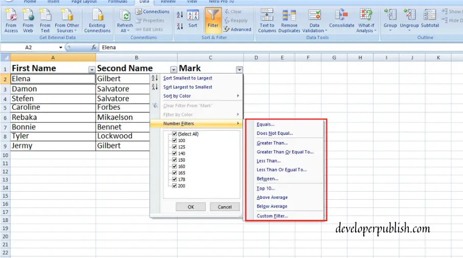
5. When you choose the Between option, it will take you to the custom filter dialogue box, in which you may filter the data as you wish.
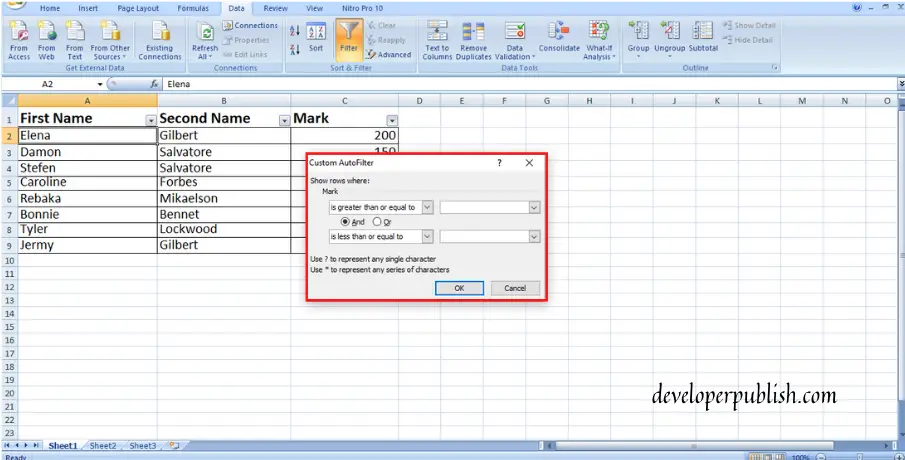
Here is an example of the Filter fuction:
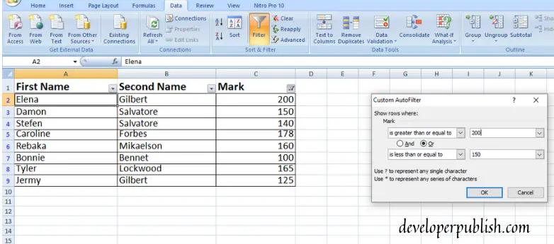
This picture displays a set of mark lists of the students. The data is wanted to be filtered and has to display the marks that are greater than or equal to 200 or less than or equal to 150. So the Filter is used.
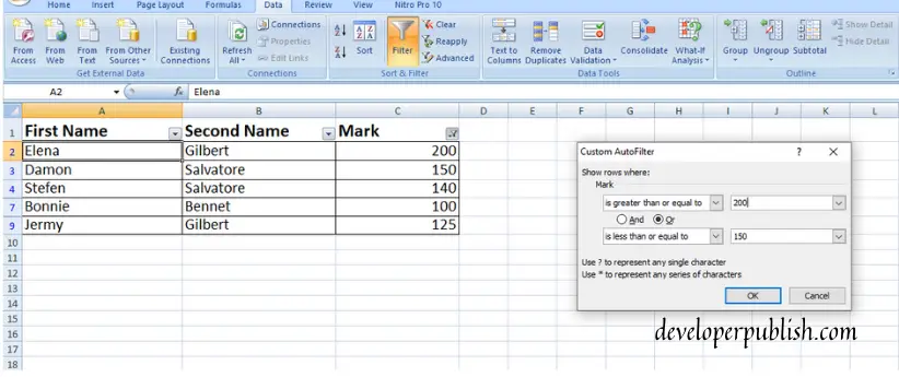
This picture displays the data that has been filtered.
This is how you use the Filter in excel. This is a common way to filter the data. If you want to filter a data that is entered in a table created in an excel sheet, you can use the same way.
Filter in table
The advantage of using a filter in tables is that, the header arrow becomes a default option in each column of the table. Also get to know how this function works in tables of excel.
- Create and format a table, enter the required data in it. You will automatically see the header arrow on top of each column of the table.
2. The header arrow is showed up in the above image, as the data has been entered a table which was created and formatted. Click on the header arrow and it will show a pop up with several options.
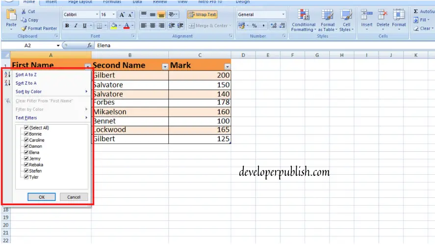
3. You will see a list of checked data, uncheck the Select All option and select the boxes that you want to show. Click OK.
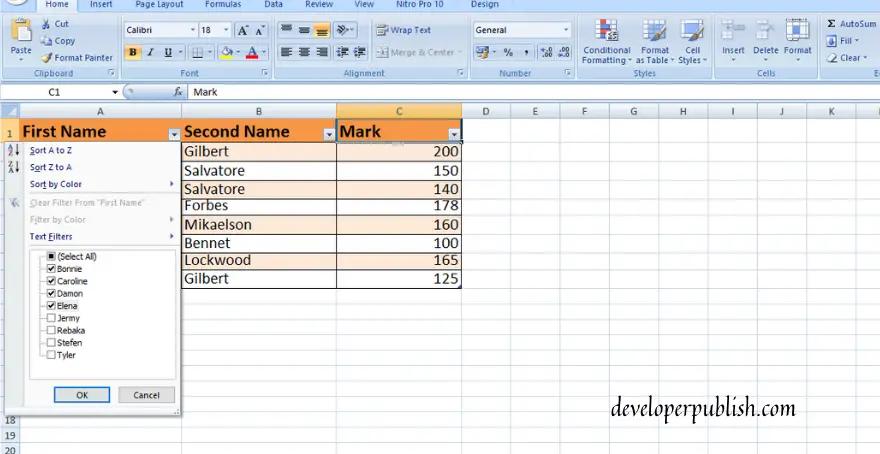
The pictures shows the selected boxes.
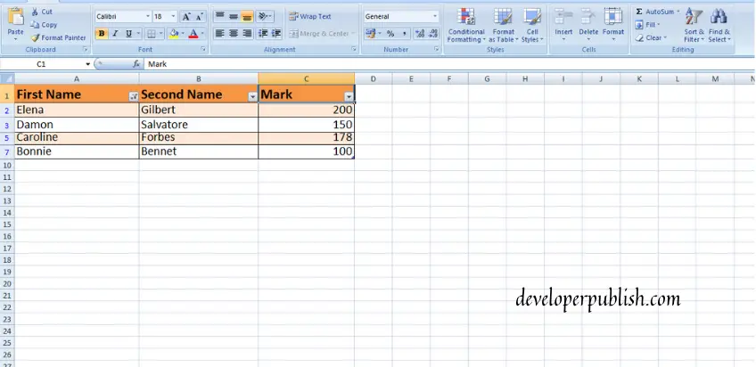
This shows the selected boxes and hided the others.
This is how the Filter in Excel works. Hope you found this post useful.


