In this post, you’ll learn a simple tip that demonstrates how to reverse a list in your excel spreadsheet.
Microsoft Excel provides various options to enter the data in a specific order. Sorting of data, sorting by color are some options that help us arrange the data in a proper list.
Arranging a list in order is quite a simple job, but reversing an arranged list must be done carefully. Excel also provides an option to reverse a list of data easily.
Reversing a list in Excel
Changing the order of an arranged data list is done by reversing them. Here is a step-by-step explanation of reversing the data is given with examples.
- Enter the numerical values in the nearby column of the data column. You can just type the first three numbers and simply drag the column to fill the rest of the values for the data.

2. After adding the numerical values for the data, select both columns. Selecting both columns is important. If something goes wrong in selecting the columns, then it might collapse the entire list of data.

3. After selecting the columns, choose the sorting option on the top right corner of the excel sheet. You will get a list of options like “Sort Ascending”, “Sort Descending”, and “Custom Sort”.
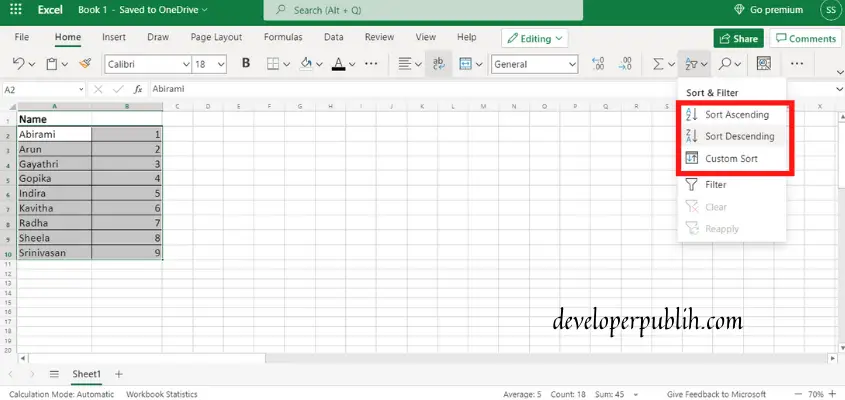
4. Choose the “Sort Descending” option to reverse the list of data. Once you choose the option, the data in the selected columns will be reversed, including the numerical values of the data.
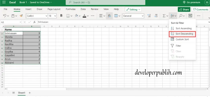
You can check the difference in the list of data in the previous picture and the above picture.
Other Ways to Reverse a List in Excel
There are other ways to reverse a data list.
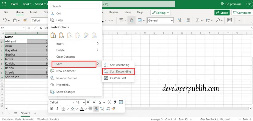
- After selecting the columns, which need to be re-arranged, just right click and you will get a pop-up. Select the “Sort” option from the list shown in the pop-up. You will get a list of sorting options, Choose the “Sort Descending” option from that. The list will be reversed.
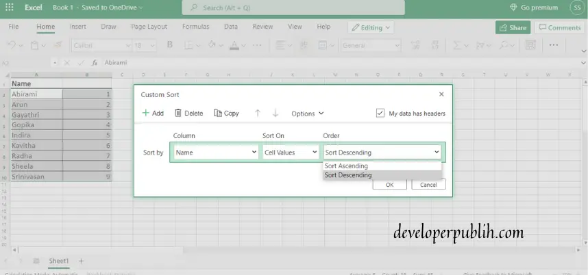
2. Or you can also choose the “Custom Sort” option and change it manually. In this option, a dialogue box will appear with few options. Fill in the required fields and click ok. Under the custom sort dialogue box, the sort by option chosen column will only be reversed.
The above options are the ways to reverse a list of data in Excel. Hope you got the information from this article.


