Address Function in Excel

In this post, you’ll learn about the address function in excel and how to use it in your excel spreadsheet.

Address Function in Excel

The function, in which the address can return the address for the cell based on the given row and column.

                          Example:ADDRESS (1,1) IT RETURNS $A$1

It is used to construct a cell reference inside a formula. To create a cell address from a given row and column. Cell address refers to the provided worksheet.

Syntax

                           =ADDRESS(row_num,col_num,[abs_num],[a1],[sheet])

It is the syntax of the address cell to access the given worksheet’s cell number. The arguments of the syntax are elaborate below.

Arguments

row_num –which is used in the cell address

column_num –which is used in the cell address

abs_num-it is an address type defaults to the absolute value

a1-it is a reference style

sheet-it will name the worksheet used in

The syntax used above gives the shortest method to word on address function on excel. The main parameters in the syntax are the row_num, and col_num others are optional in this address cell.

CODE OF THE EXAMPLE:

In this, I have given the row and column and found out the address of the given cell.

How to use Address Function in Excel?

In this, we are going to apply step by step process for addressing the function.

open Microsoft Excel and start with the worksheet.

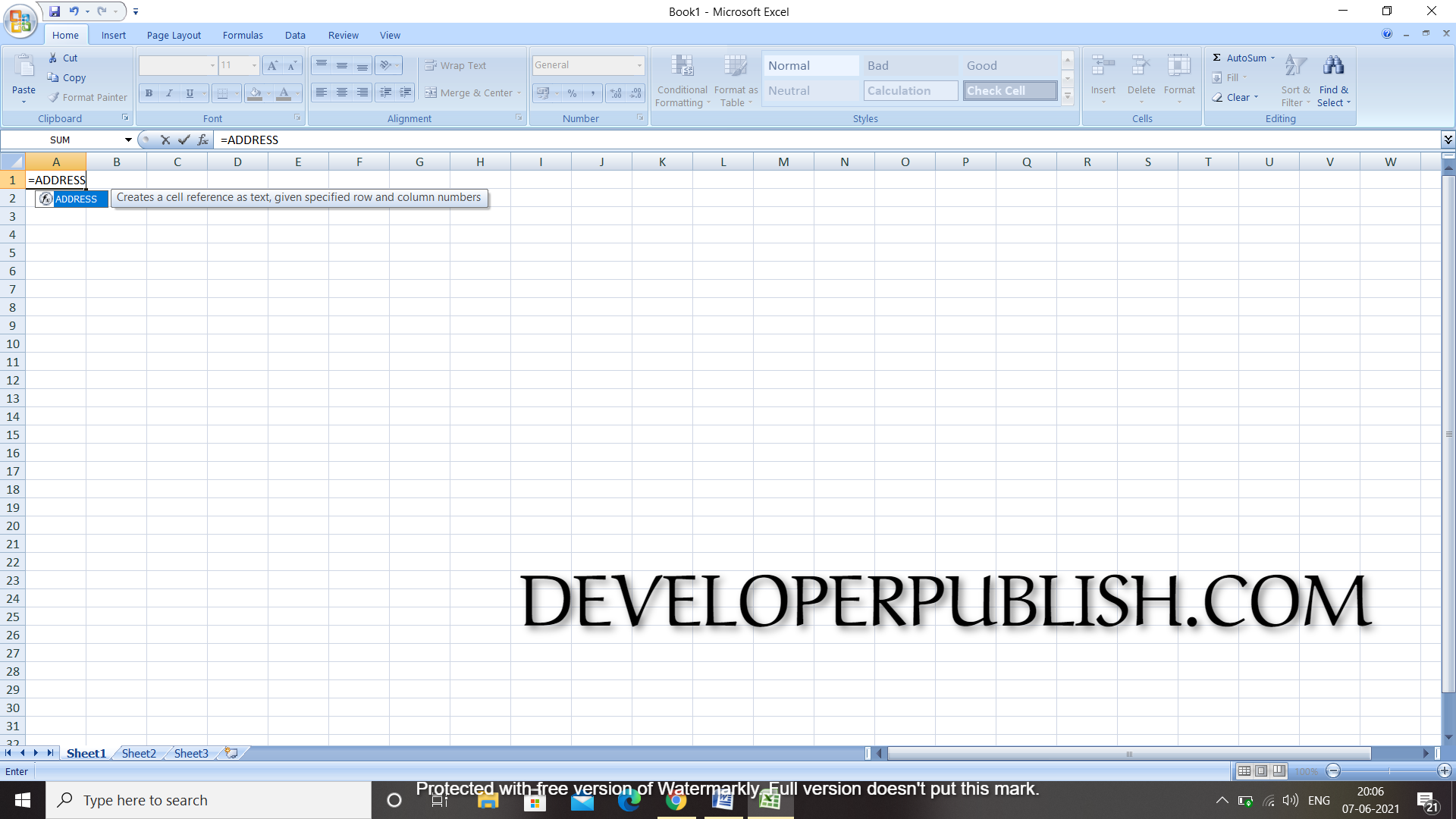
Step 1: type =ADDRESS in the first cell to create a cell reference as text is specified row and column numbers.

Step 2:As the syntax of the argument is explained clearly, open the brackets accordingly,

Step 3: Now, enter the row number and column number to the cell reference.

Step 4:So, I have entered the row and column number as 2,2 now, if I give a comma again over 2, the cell moves to the next step to find whether it is absolute or relative to row and column each has a value of 1-4 the choice is based on us.

Step 5:Now, if we place a comma again, it will show the option as address style in which it can talk about the references and column name and row name. Now I’m selecting the one to speak about the name of the row & column.

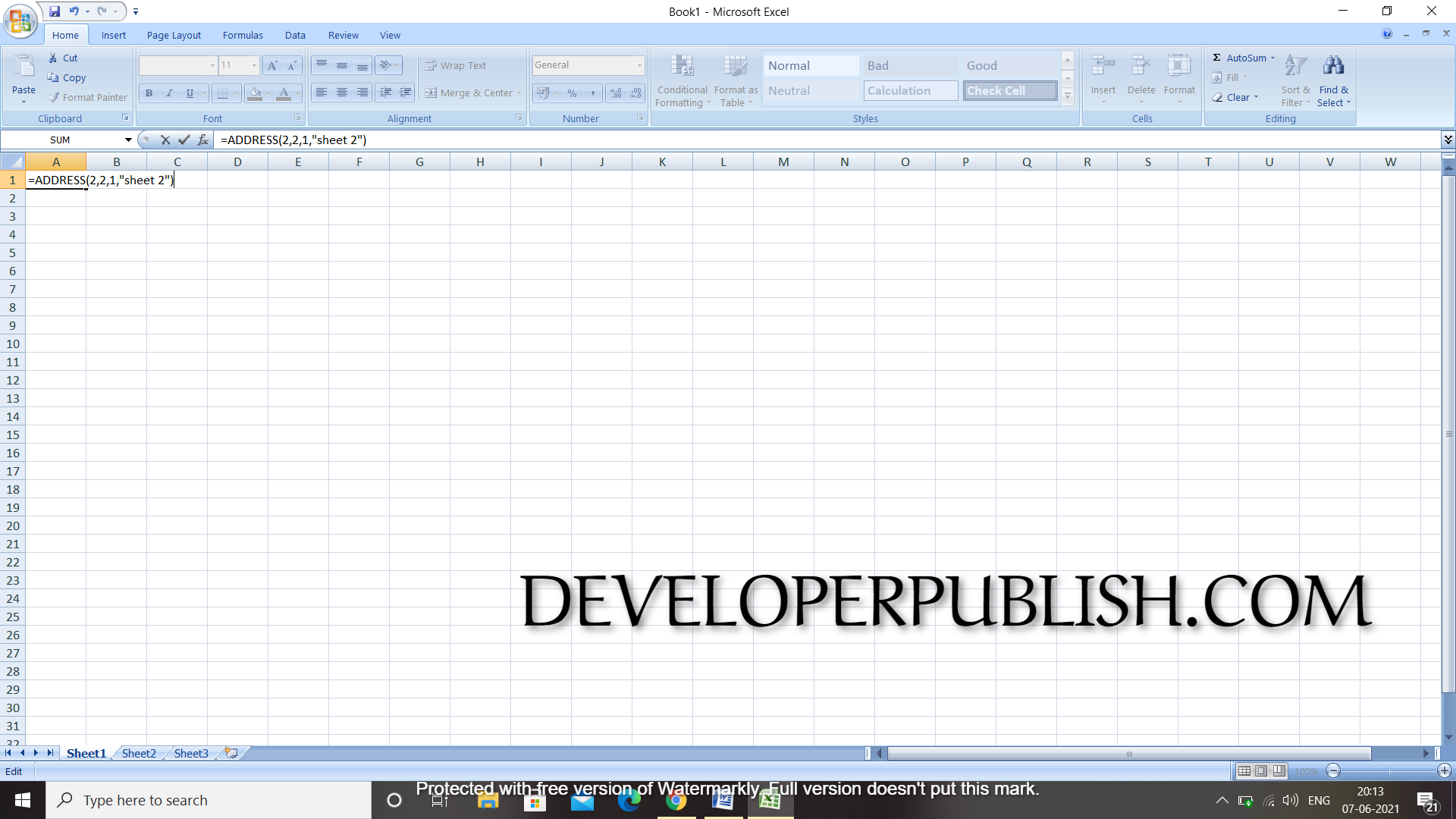
Step 6:This is the final parameter of the syntax which can be given in “………” (double quotes)and close the bracket.

Double click it and you will get the cell name.