How to Perform a Case-Sensitive Lookup in Excel?

In this post, you’ll learn how you can perform case sensitive lookups in Excel when using VLOOKUP.

Case-sensitive lookup in excel

In default, the lookup value in the VLOOKUP function is not case sensitive, i.e., it’ll return the first matching value irrespective of the case.

Making VLOOKUP Case Sensitive

In the table given below:

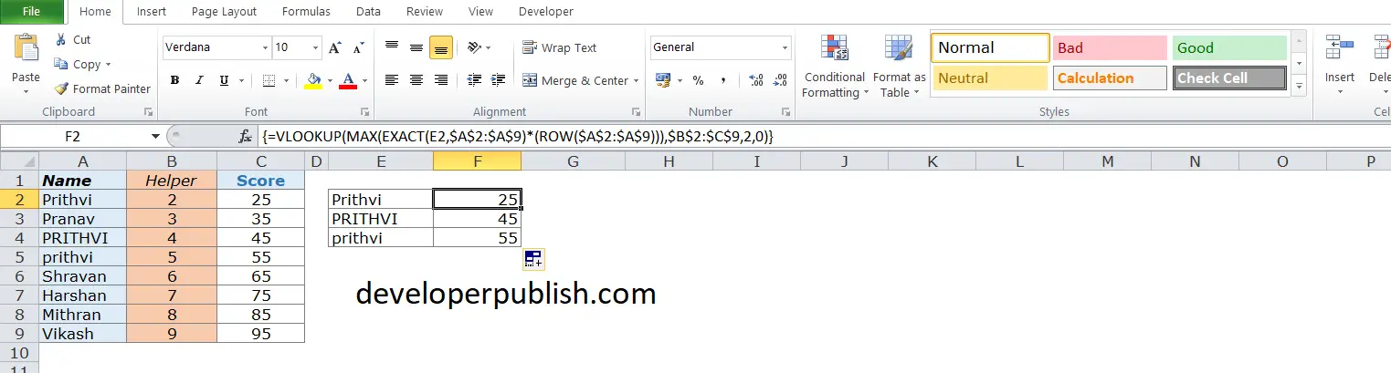
As you can see, there are three cells with the same name (A2, A4, and A5) with a different letter case.

E2:F4, we have the three names Prithvi, PRITHVI, and prithvi along with their scores.

Making VLOOKUP Case Sensitive – Using Helper Column

A helper column is used to get the exact lookup value for each item in the lookup array. This will help in differentiating between names with their letter case.

Follow these steps:

• Insert a helper column to the left of column C.
• Here, we are inserting the helper column between columns A and C.

• In the helper column, enter the formula =ROW(). It’ll insert the row number in each cell.
• Use the below formula in cell F2 to get the case-sensitive lookup result.

=VLOOKUP(MAX(EXACT(E2,$A$2:$A$9)*(ROW($A$2:$A$9))),$B$2:$C$9,2,0)

• Copy and paste it for the remaining cells (F3 and F4).

Note: Since this is an array formula, use Control + Shift + Enter instead of just enter.