In this post, you’ll learn about a chart in Microsoft Excel called the Gantt Chart. Also, it helps you demonstrate how to make a Gantt Chart in your Excel worksheet.
What is Gantt Chart ?
Gantt Chart is one of the best types of charts in Excel. This chart type is helpful for project management. In this chart, we can schedule the tasks so that we can accomplish them well. Excel provides an Gantt chart template which you can directly use it in your spreadsheet.
How to Make a Gantt Chart in Excel?
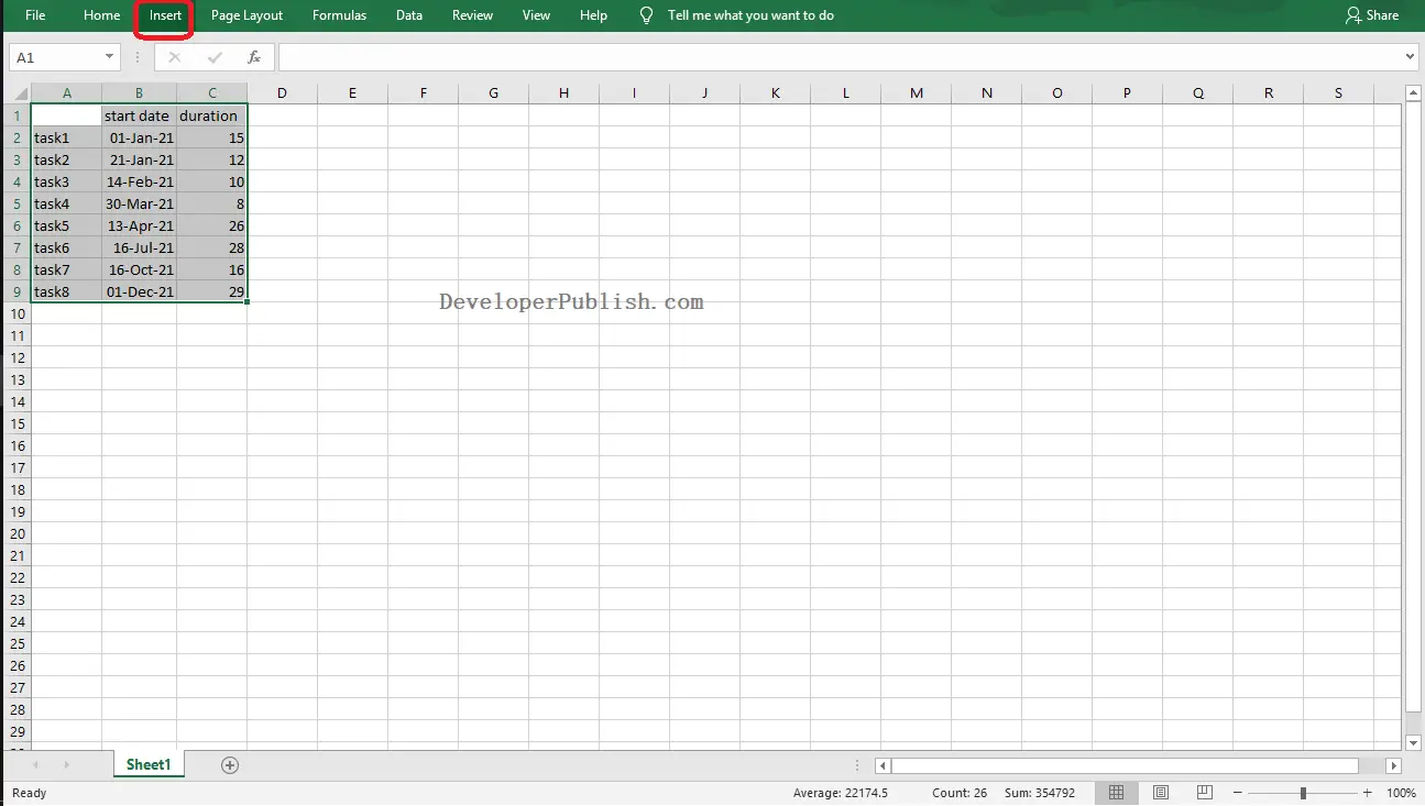
- To get started, select the data to create a Gantt chart.
- Go to the Insert Tab, select the Insert Column or Bar Chart icon from the Charts group.
- Now, select the stacked Bar chart type from the 2-D bar category.
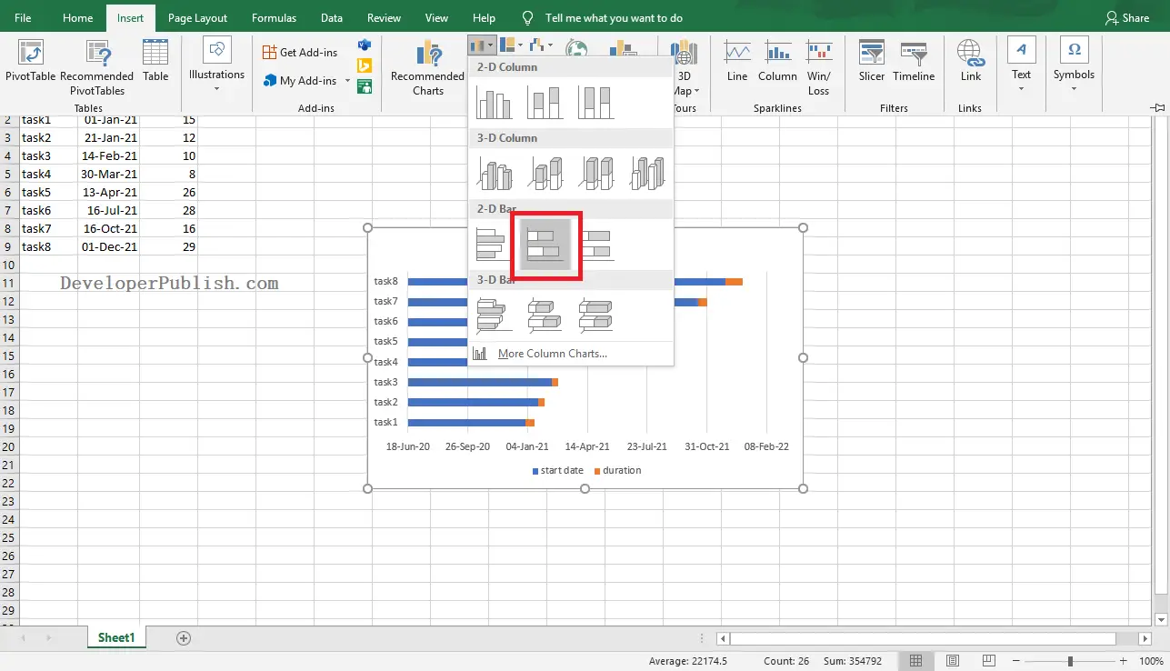
- You will get a bar chart as in the below image.

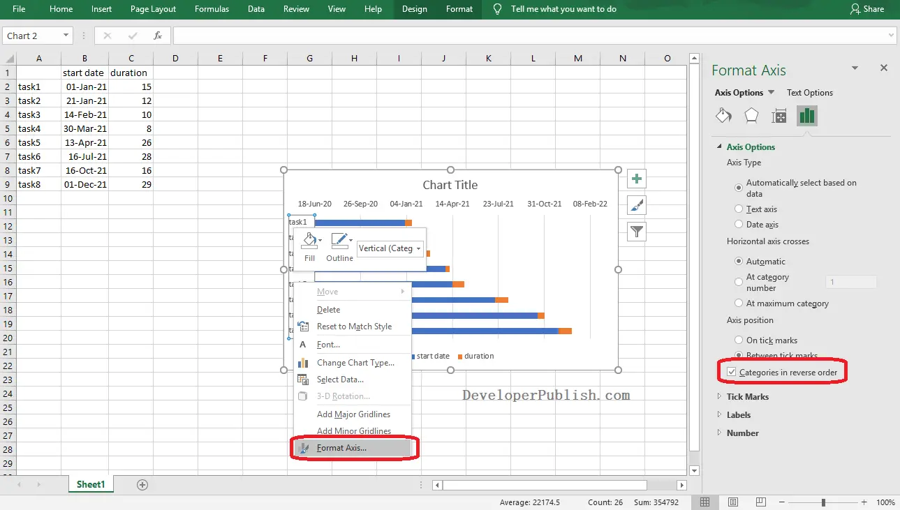
- To arrange the tasks in ascending order, right-click on the vertical axis. Then, select the Format Axis option from the pop-down menu.
- In the Format Axis pane, select the Categories in reverse order check box.
- Add the chart title and remove the legends if you want.
- Now, right-click on the blue bars and select the No Fill option from the Fill icon.
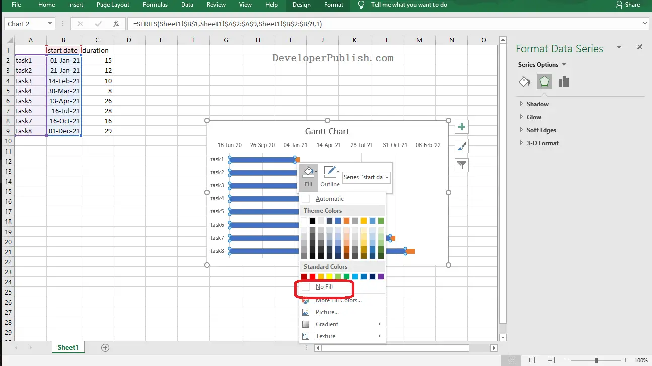
- Also, select the No Outline option from the Outline icon.
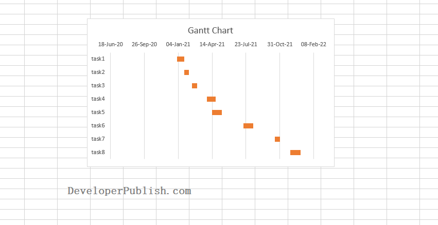
You can see the created simple Gantt Chart in the worksheet as in the above image.


