In this post, you will be guided through simple and easy-to-follow steps on how to use the FVSCHEDULE function in Excel.
Microsoft Office Excel provides the FVSCHEDULE function, which helps to calculate the future value of an investment with a variable interest rate. It returns the future value of a single sum based on a schedule of given interest rates.
FVSCHEDULE Function in Excel
FVSCHEDULE is used to calculate the future value of an investment with a variable or adjustable rate. It returns the future value of an initial principal after applying a series of compound interest rates. This is a built-in Excel function under the Finance category.
FVSCHEDULE Syntax
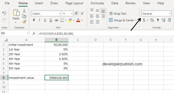
=FVSCHEDULE(principal, schedule)
The FVSCHEDULE function and arguments
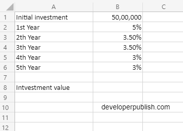
- principal (required) – The initial investment sum.
- schedule (required) – Schedule of interest rates, provided as range or array.
How to use the FVSCHEDULE function in Excel?
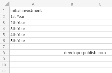
- Open Microsoft excel and launch a workbook or create a new Excel sheet.
- As said in the description, you need the values of all the above arguments to carry out the FVSCHEDULE function and get the correct and Investment value.
- Enter the arguments in the same order of the syntax, one below the other, as shown in the picture below.
- At this time, in a similar way enter the values of each of the arguments in their corresponding adjacent cells in the worksheet.
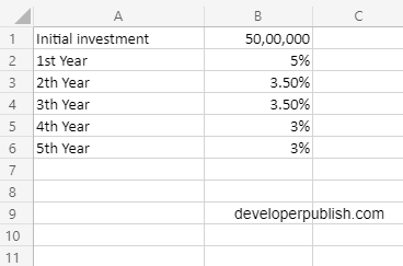
- Below the tabulated list of arguments, select a cell and enter “Investment value”, the cell to the right will display the value of the formula (making identification easier).
- When entering the formula, always start with the “=” operator. After entering the “=” operator enter FVSCHEDULE to initiate the formula followed by an open parenthesis. Excel recognizes “=’ as the start of a formula, if not included, excel will not accept and evade the execution of the function.
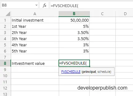
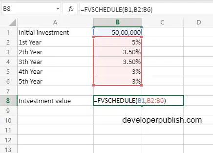
- With the parenthesis open, select the arguments in the order of syntax. The position of the cell will be visible in the formula. Here, as the argument values are entered in a group, use the fill handle to enter the values. The change in color of the cells aids to identify the name and of the cells in the formula.
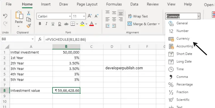
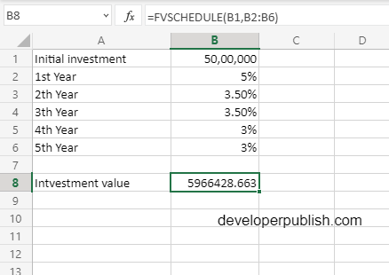
- To conclude, close the parentheses and click enter. The cell which contains the formula will display the Interest value. The value will be displayed in numerical form, where we should convert it into currency.
- To convert the from numerical form to currency, first select the cell with the value, under the home tab, open the drop down box and click currency icon. The selected cell value will change accordingly.