AVERAGEIFS Function in Excel

In this post, you’ll learn about AVERAGEIFS Function in Excel, its syntax and the way of using AVERAGEIFS Function in Microsoft Excel spreadsheet.

What is an AVERAGEIFS Function?

An AVERAGEIFS Function is also one of the statistical functions. AVERAGEIFS function calculates the average of numbers in a range even in a multiple criteria.

The criteria used for AVERAGIFS can include logical operators such as (<, >, <>, =) and wildcards (*, ?) for partial matching. AVERAGEIFS was introduced in MS Excel 2007.

SYNTAX:                      

= AVERAGEIFS(average_range, criteria_range 1, criteria 1, criteria_range 2, criteria 2…)

Expressions:

• = – built-in function.
• AVERAGEIFS() – Function name.
• average_range – the range(variations) to average.
• range 1(required value),range 2[optional] – the range arguments to calculate.
• criteria 1(required argument), criteria 2[optional] – the criteria(standard) to use on range.

average_range – the arguments include numbers, names, arrays that contain numbers.

Criteria – can be from 1 to 27 in the form of a numbers, expression, cell reference, or text that refers the cell.

AVERAGEIFS Function is in a group of eight functions in Excel. It splits logical criteria into two parts(range + criteria). AVERAGEIFS requires a cell range for range values, but you cannot use an array. It also ignores empty cells automatically, even criteria matches.

NOTES:

• The order of argument is different between the AVERAGEIF and AVERAGEIFS. The range of average is always the first argument in AVERAGEIFS.
• #DIV0! Error returns when there is no match in the criteria.
• All the additional ranges must have the same numbers of rows and columns as the average_range.
• Non-numeric values must be enclosed within the double quotes.
• The wildcards characters (?) and (*) can be used in criteria.

                            A question mark(?) matches any one character.

                            An asterisk(*) matches zero or more character.

                            By using tilde(~) you can find the literal (?)question mark or (*)asterisk (~?, ~*).

The Main Difference between AVERAGEIF and AVERAGEIFS Function is;

How to use AVERAGEIFS Function in Excel?

AVERAGEIFS Function is a built-in function which is a worksheet function(WS) in excel.

Multiple criteria:

The values must be in pairs[range, criteria].

DOUBLE QUOTES (“”):

• Text values is must be within double quotes, but numbers are not. If the logical operator with a number, the number and operator must be within double quotes.
• Value from another cell – value from another cell by using catenation.
• WILLCARDS:

The wildcards characters question mark (?), asterisk (*), or tilde (~) can used in criteria.

• The question mark (?) matches any single characters.
• The asterisk (*) matches any sequences of characters.
• The tilde (~) is an escape character it allow you to find the literal wildcard.

Step 1:

Open the workbook in your Microsoft Excel.

Step 2:

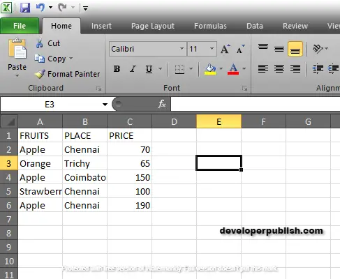
Enter the data, in the workbook.

Step 3:

In this example, there are two conditions specified in the list. One is fruits and the other one is places also with the price amount according to the places. We can calculate AVERAGEIFS Function for ‘Apple’

In this example, there are three times apple is specified in the data which is situated in Chennai, Coimbatore and again in Chennai with the price amount of Rs. 70, 150, 190.

STEP 4:

Now you are going to calculate the AVERAGEIFS of apple located in Chennai.

STEP 5:

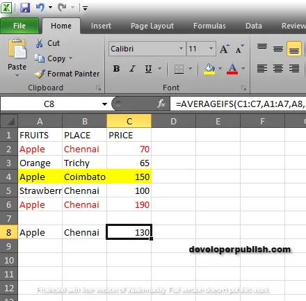
In the new cell, give the formula of the function or the syntax . Start with ‘ =’ which is common for every functions, AVERAGEIFS to initiate functions name, followed by open parenthesis. According to AVERAGIFS Function , the first step is to calculate average_range.

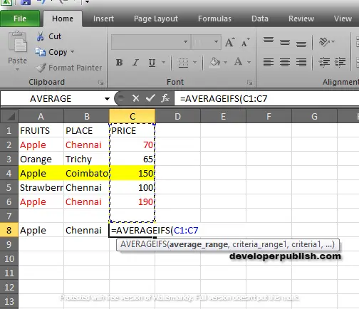
In this example, the average_range is PRICE(C1:C7).

STEP 6:

After calculating the average_range, put a comma and the next step is to calculate is criteria_range 1.

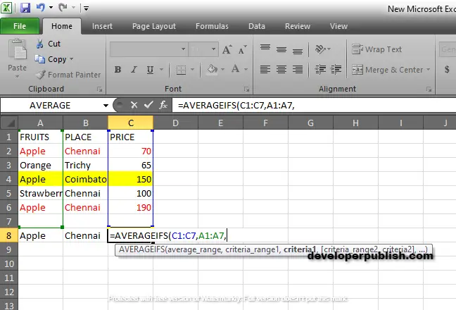
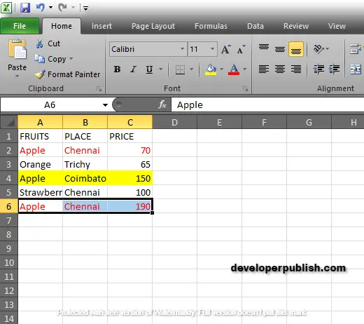
In this example, the criteria_range 1 is apple, so first we are selecting the fruits. Now the values of the criteria_range 1 is FRUITS(A1:A7).

STEP 7:

After calculating criteria_range 1, keep a comma and start with the next step. The next step is to calculate criteria 1.

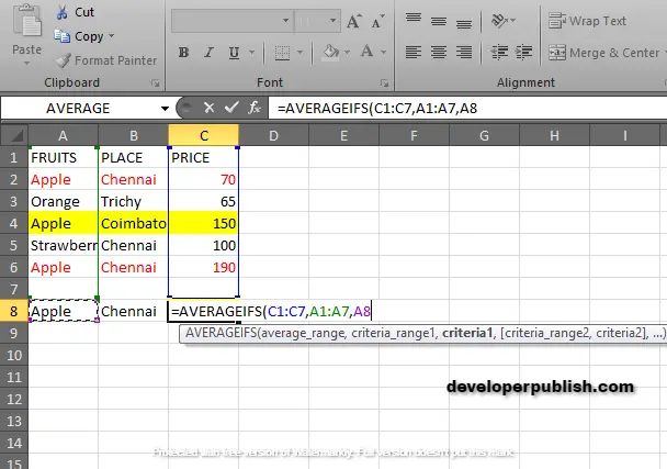
In this example, the value of criteria 1 is apple, so you can select apple in row A8.

STEP 8:

After calculating criteria 1, keep a comma. The next step is to calculate the criteria_range 2.

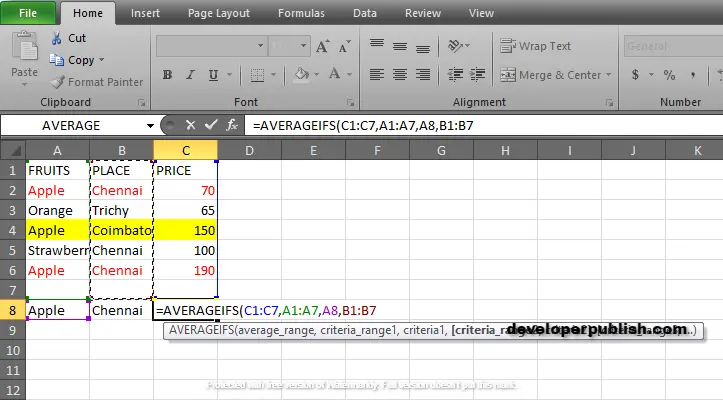
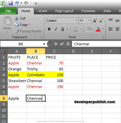
In this example, the criteria_range 2 is places, so we select places(B1:B7).

STEP 9:

After calculating criteria_range 2, keep a comma. The next step is to calculate criteria 2.

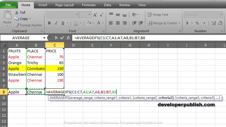
In this example, criteria 2 is the place Chennai.

STEP 10:

Press enter to get the calculated results.