In this post, let’s learn how the TRIM function works in excel, describe the formula syntax, and how you can use the TRIM function in your spreadsheet.
What is TRIM Function in Excel?
The TRIM Function in Excel is used to remove the extra spaces in data and leaves a single space between words. It is a TEXT Function.
Syntax of TRIM Function
=TRIM(text)
Parameter
Text-(Required) The text from which you want to remove extra spaces.
Example
=TRIM(R8)
=TRIM(“hi welcome”)
How to use TRIM Function in Excel?
The following steps will explain the work of the TRIM function in an excel spreadsheet:
- Create an Excel spreadsheet with the required data in it.
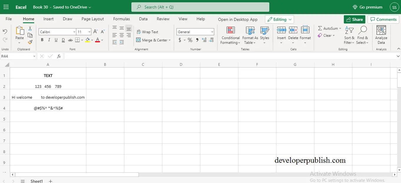
- Here, we enter the syntax of the TRIM Function on the cell where you want to display the spaces removed text.
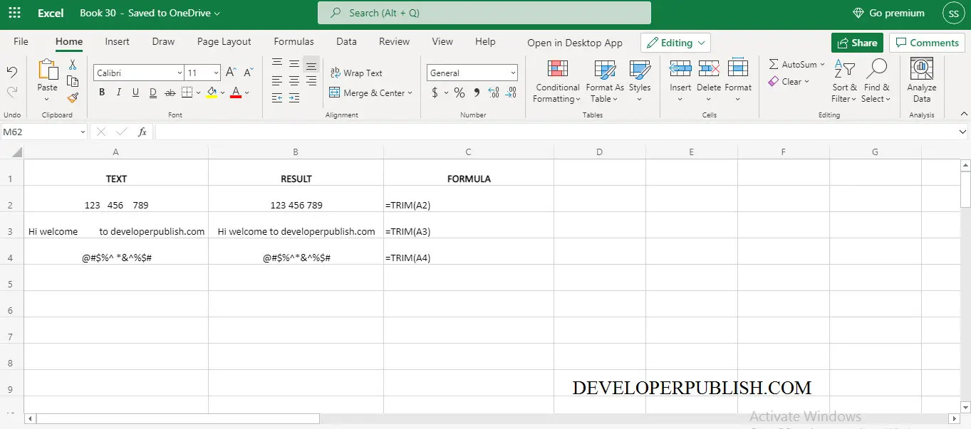
- In cell A2 we have performed TRIM Function works on numbers.
- Text: 123 456 789 Result: 123 456 789 Formula: =TRIM(A2)
- It works same on the text and symbols.
Note:
The TRIM Function only removes the ASCII space character from the text.


