In this article, you’ll get to know how to format cells which has text to a number in Microsoft Excel.
How to format cells in Excel?
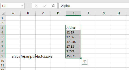
- Select the cell which you want to format.
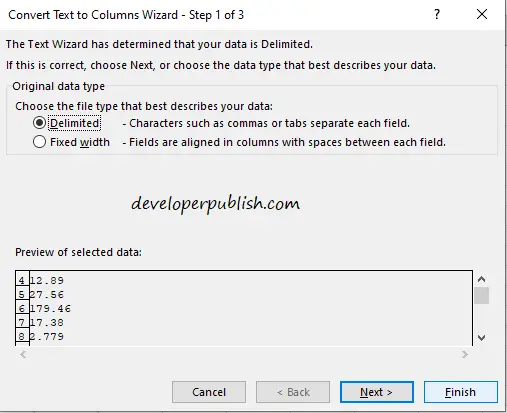
- Go to Data in the Menu tab and select Text to Columns in the Data Tools group.

NOTE: This works only if you select cells in the same column.
- When the Text to Columns dialog box opens up click on Finish to proceed.
Now set the format by opening the format dialog box using Ctrl+1, or right-click method.
- Select Number in the Categories.
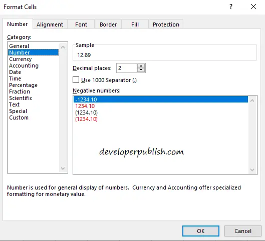
- After selecting the format click on OK to save the changes.
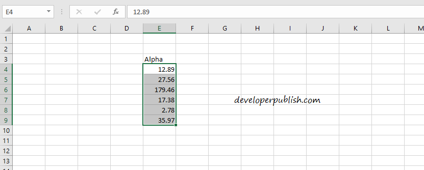
Now the cells are formatted.
Formatting using a Function
Another to format your cells is by using the VALUE function.
The syntax of the function is =VALUE(cell reference).
You can enter this function in the formula bar of a new cell or a range of cells besides the original one.
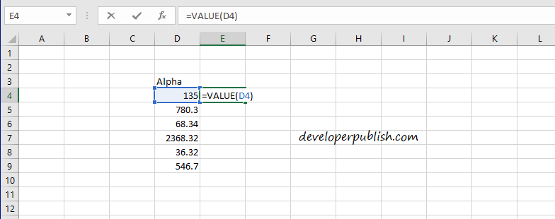
For a single the value will appear when you enter the function just for it.
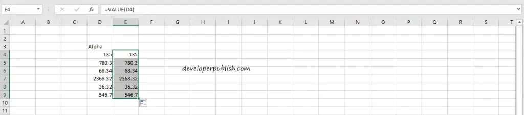
In the case of a range of cells, you’ll find a plus symbol in the bottom-right corner of the cell which has the function and now click on that and drag it over to the range of cells below it.
Now the cells beside the original ones will also have the formatted value.
This is how you format cells in Excel.


