Summarizing with Blank Cells in Pivot Table
In this post, you’ll learn about summarizing with blank cells in Pivot table in your Excel spreadsheet.
Summarizing with Blank Cells in Pivot Table
While working with a large set of data, it is possible to have blank cells in the data. It is bit difficult to summarize a table with blank cells or non-numeric values in the table. But, excel pivot has a feature to summarize these fields. It can be done with the help of count function.
Count Function
When fields with non-numeric or blank cells are added to the fields, count function is the default summary function for the Pivot table.
The pivot table Count Function summarizes the following values:
- text
- numbers
- errors
It does not count the blank fields. But to count the blanks in the table, you can alter the pivot table.
Look at the example below
- It is a collection of data of products sold in a day with their quantities.
- We could see that certain cells are blank.
- So, when we insert a pivot table for the data, the pivot table, by default summarizes the data using the count function as there are fields empty.
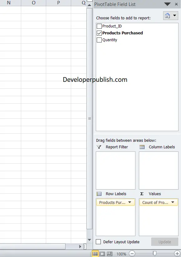
- After inserting the pivot tables, check the products and the quantity fields in the fields pane bar.
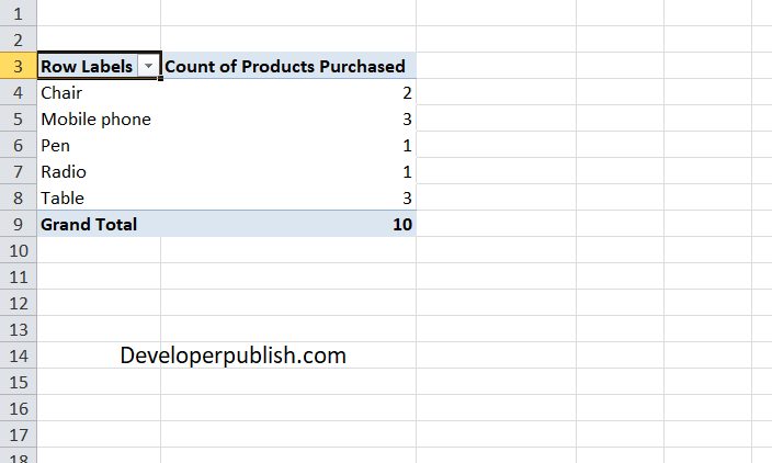
- We are going to count the products and how many times they are sold in the day.
- While looking at the data in the pivot table, we can see that these are not legit values as the blank fields in the original data are left out.
- To avoid this, we are going to uncheck the quantity column and drag the products column into the value field in the pane.
This will give you the exact count of each product.


Leave a Review