Summarize by Average in Excel Pivot Table
In this article, you will learn how to summarize by Average in Excel Pivot Table and how this functionality can be used with-in your Excel worksheet.
Summarize by Average in Excel Pivot Table
Excel offers you a variety of methods to summarize your data in Pivot table. Some of its summarize functions are Sum, Min, Max and Average.
Whenever you place a field in the ∑ Values in the field list pane, it automatically sums the value in the column. The default function for the numeric value fields in the PivotTable is the Sum function, but you can choose a different summary function.
Now Let us see how to summarize by Average in Excel Pivot Table.
Take a look at the given example.
It is a sales report for different months of the year.
- Now, insert a pivot table by clicking the insert tab in the ribbon and click the pivot table option.
- Insert the pivot table in a new worksheet.
- Choose the fields for your pivot table from the pane.
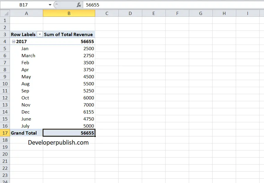
- By default, the pivot table summarizes the whole column and gives the total value in the grand total field.
- In the PivotTable, right-click on the Grand Total field, and then click Summarize Values By.
- From the drop-down menu, click on the Average function.
- Now you can see, the grand total will show you the average sales revenue.


Leave a Review