Subtotals and Grand totals in Excel Pivot tables
In this post, you will learn how to add Subtotals and Grand totals in Excel pivot tables and how to use it with-in your excel spreadsheet.
Subtotals and Grand totals in Excel Pivot Tables
A pivot table normally summarizes the given values and displays them at the grand total field. The summarizing functions can be changed from the value field settings.
Now, let’s see how to add subtotals and grand totals manually.
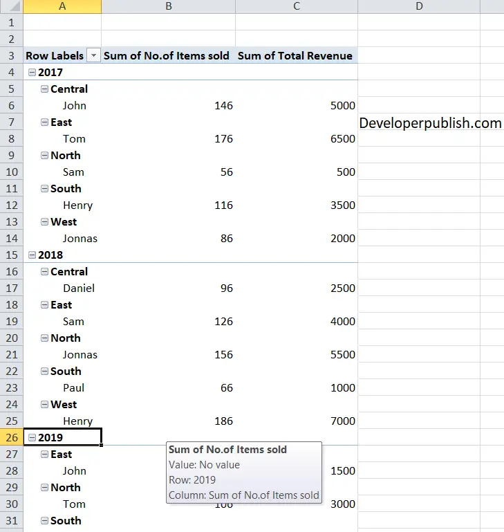
Look at the following example,
The sales report of a firm is given in the form of nested fields in the pivot table.
To add the sub total field to the table,
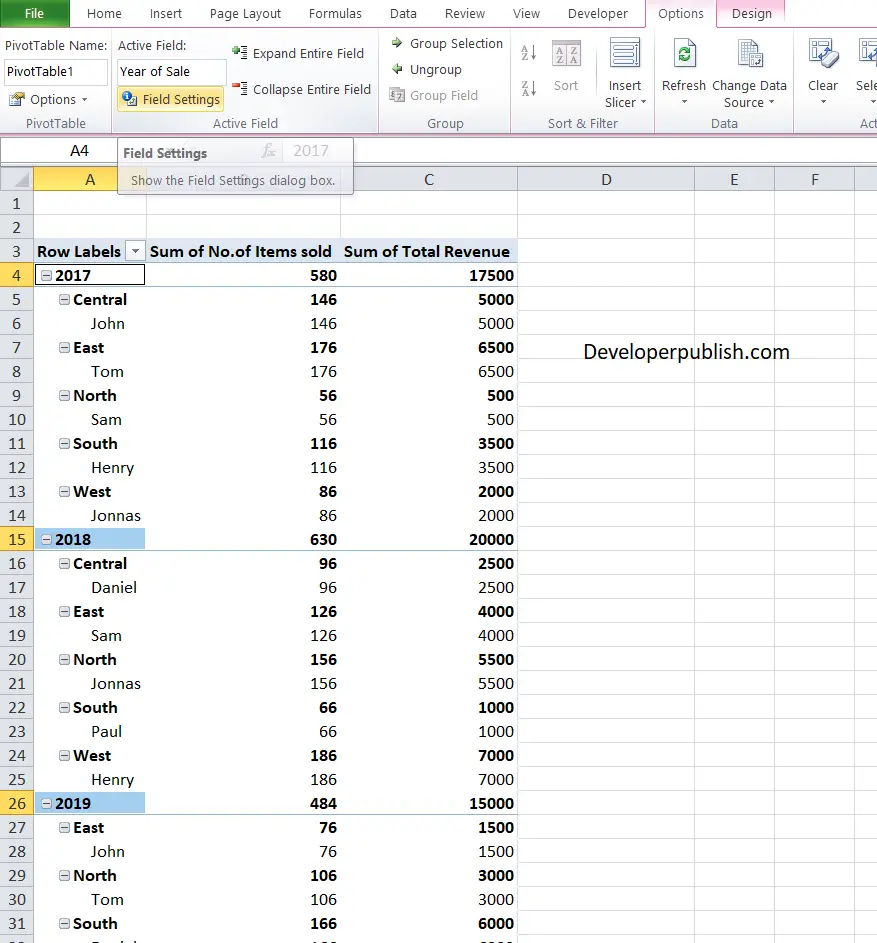
Click on the subgroup of the table and on the Options tab click on Field settings.
This will display the field settings tab and on the Subtotals section check the automation option.
Click ok
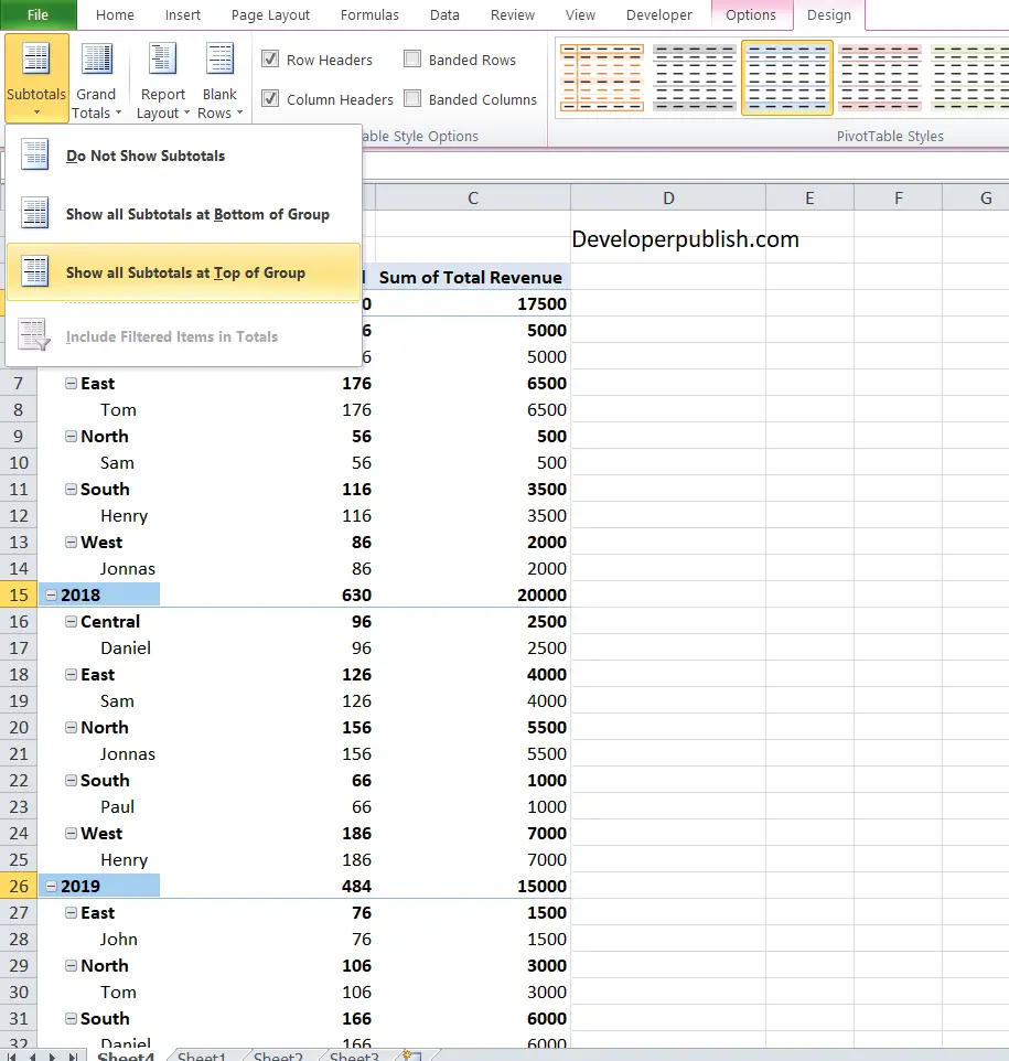
Now click the sub group and click the design tab in the ribbon.
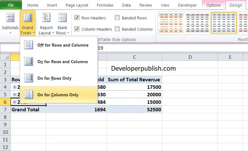
The first two options or icons available in design ribbon are Subtotals and Grand totals.
First click on subtotals and in the drop down menu choose the orientation of the subtotals that needs to be displayed.
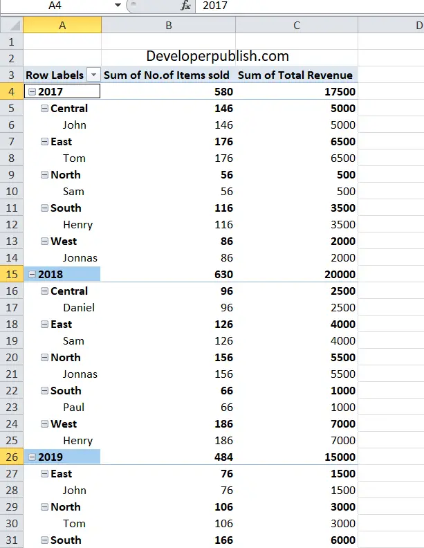
Select an option and the subtotal is displayed on the pivot table.
Now click the Grand totals drop-down and choose an option from it.
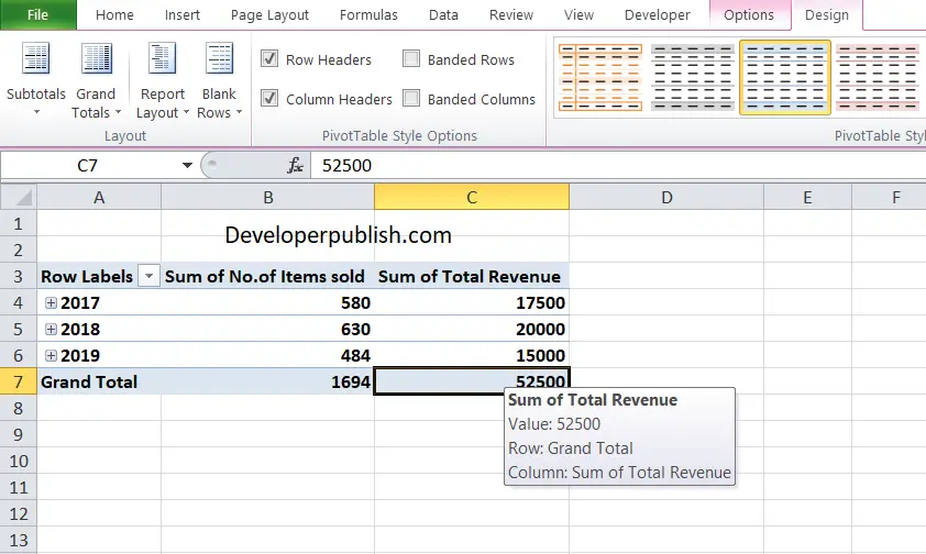
The pivot table shows the grand totals depending on the option you selected.
You can see that, the grand total is displayed at the bottom of the Pivot table.






Leave a Review