Slicers in Excel Pivot Table
In this post, you’ll learn about Slicers in Excel Pivot Table and how to use them in your Excel workbook.
Slicers in Excel Pivot Table
Explore how you can use and adjust slicers in Excel Pivot Table
What Is A Slicer In Excel?
By definition, a slicer is an object in Excel that allows you to filter your data. Slicers can be used with both Tables and Pivot Tables. It is commonly used in pivot tables.
Basically, the slicer filters the data based on the requirements and gives you a clear and precise flow or report. The buttons in the table are used to toggle the active filtering of the data set.
The slicer tab is displayed in the spreadsheet grid and will always be visible and available to use.You can connect multiple slicers to multiple pivot tables.
How to Insert a slicer in a Pivot table?
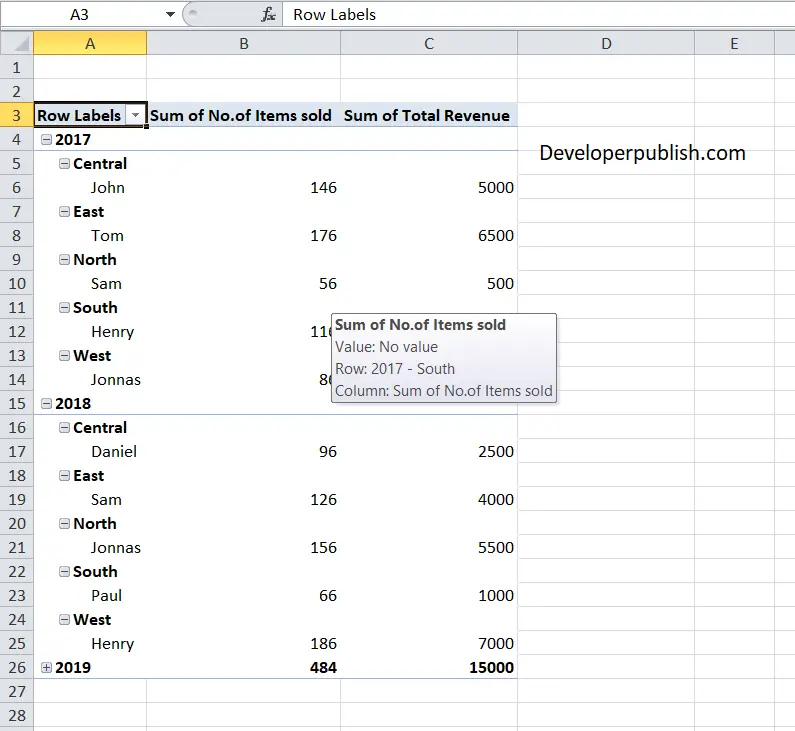
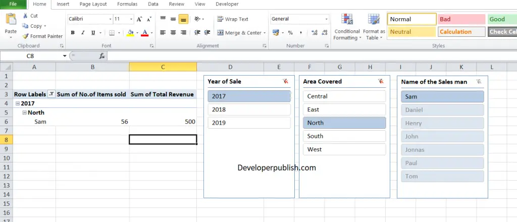
Take a look at the example below,
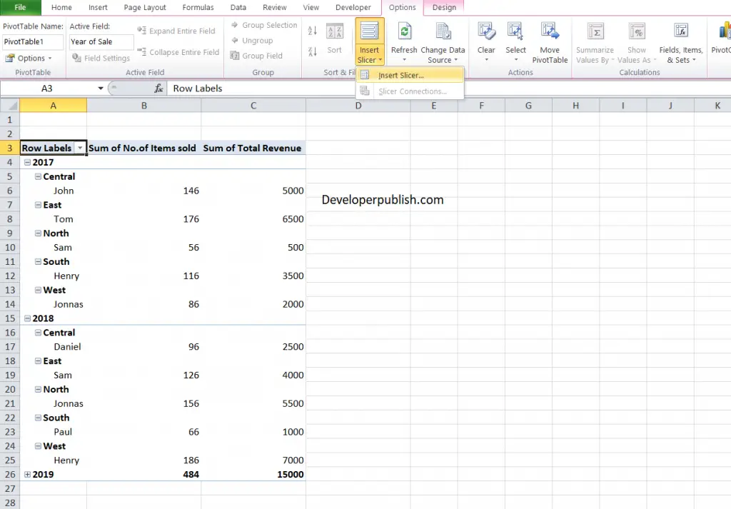
To insert a slicer, execute the following steps.
- Click any cell inside the pivot table.
- Under the options tab in the ribbon, from the Filter group, click Insert Slicer.
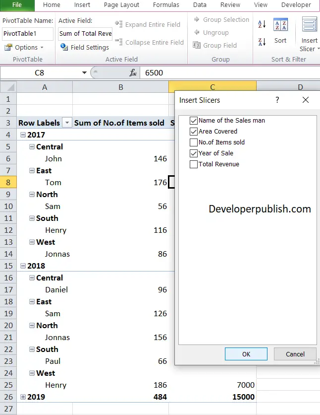
- Check the required labels and click okay.
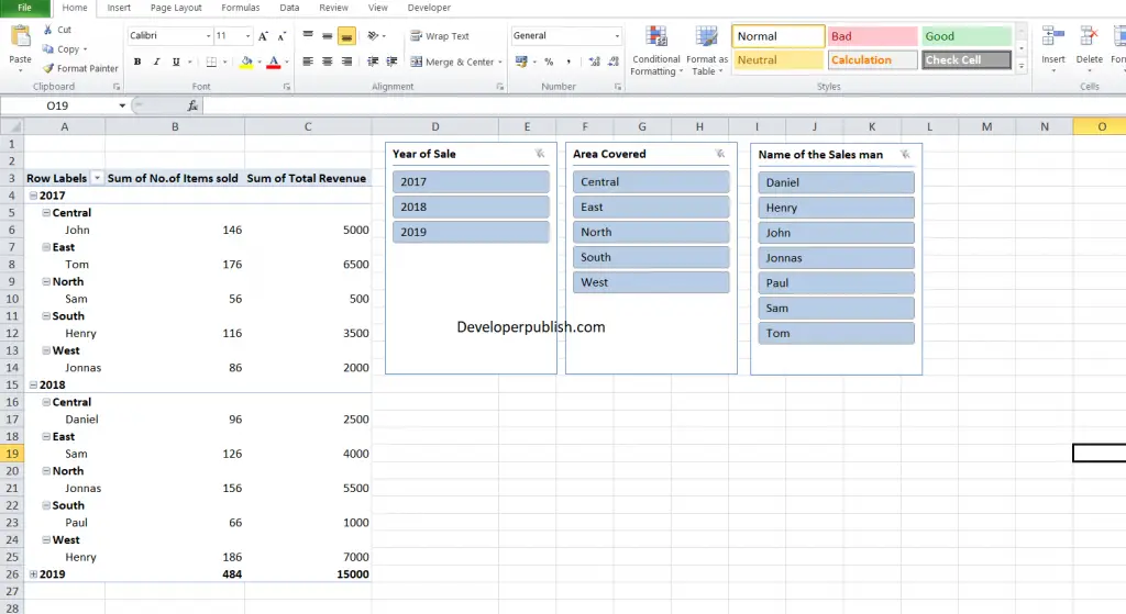
- This will insert the slicer menu in the Worksheet.
When you click on the year, the pivot table shows the data for the particular year.
When you click on the particular region covered, you will get the person covering that region in that particular year.
So slicer is a kind of filter that is more efficient than standard filters.



Leave a Review