In this post, let’s learn how the RRI Function works in excel, describes the formula syntax, and how you can use the RRI Function in your excel spreadsheet.
What is RRI Function in Excel?
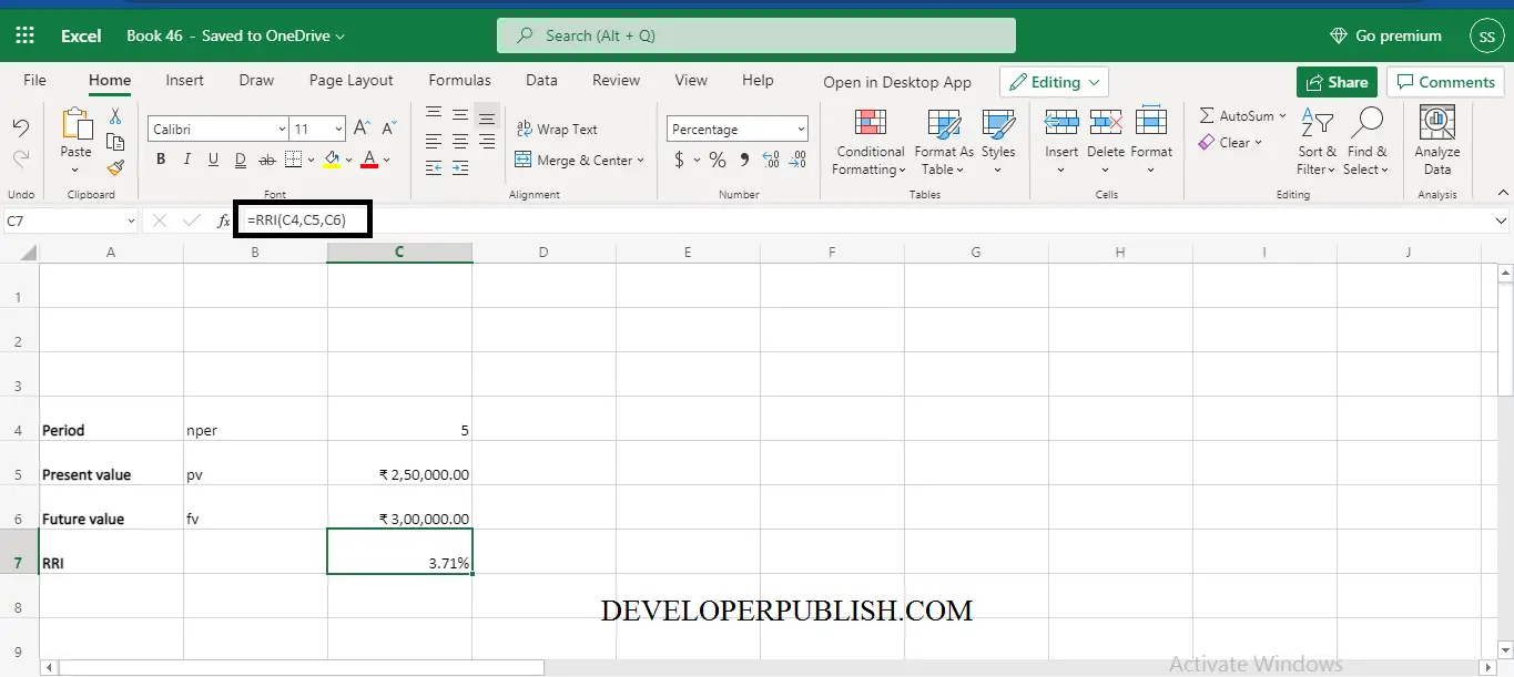
The RRI Function in Excel is employed to calculate the same rate of interest for the expansion of an investment.
Syntax
=RRI (nper,pv,fv)
Parameter
- Nper– Total number of periods to invest.
- Pv– The present value of the investment.
- Fv– The future value of the investment.
Example
=RRI (C12, C13, C14)
=RRI (B12, C13, D14)
How to use RRI Function in Excel?
The following steps will explain the work of the RRI Function in Excel spreadsheet:
- First, prepare an excel spreadsheet with the specified details in it, or open an existing file.
- To perform the RRI Function you need the parameters described in the description.
- Enter those values in cells and enter the command RRI followed by the “=” operator within the parenthesis enter the parameters.