In this post, you’ll learn about Pivot Table in Excel and how you can use it with-in your Excel spreadsheet. This article will cover the following topics:
What is a Pivot table?
Pivot table is a powerful tool, which supports calculating, summarizing, and analyzing the data and gives an interactive view to your data. Using the pivot table we can analyze the static data from a whole new perspective. We can group, break down, classify into categories and even build charts from the given data using a pivot table.
The pivot table allows us to convert the rows into columns and vice versa. Using pivot tables we can perform operations like sort, summarize, re-organize, count, group, total or average functions for a preferred set of data at a minimal effort. It is a perfect solution to analyze and report a large set of data. The best part of Pivot tables is it requires a minimal formula or no formula at times.
Pivot tables are most commonly used in situations where data needs to be aggregated and operated for analysis. It’s quite useful to calculate and summarize data while making comparisons
Key Features of PivotTable
- Analyze data at ease.
- Analyze and view data in a whole new perspective
- Filters data on specific requirements
- Precise data comparison
- Easy identification of errors
- Data patterns, data trends, and relationships.
PivotTable Terminologies
| Keyword | Description |
|---|---|
| Report filter | Report filter applies a filter to an entire table. |
| Column labels | One or more columns in the pivot table can be filtered using column labels. |
| Row labels | One or more rows in the pivot table can be filtered using row labels. |
| Values | ‘Values’ takes a field that has numerical values in it, which can be used for different types of calculations. |
| Column field | Column fields are the ones which has a column orientation in the pivot table. Each item in the field occupies a column and it can be nested. |
| Data Areas | Data areas are the cells in the table which contains the summary data. Sum, average, count, etc., are several ways to summarize the data. |
| Grand totals | Any row or column that displays totals for all cells in a row or column is called Grand totals in the pivot table. |
| Group | It is the collection of items that were treated as a single item. In excel, you can either group the items manually or automatically. |
| Item | Any element in the field that appears to be a row or column header in a pivot table is called an item. |
| Refresh | Just by the term, it is used to recalculate or refresh the table after considerable modifications to the source data have been made. |
| Row field | Any field that has a row orientation in the pivot table is called a row field. Each item in the field occupies a row and it can be nested. |
| Source data | It is the raw data or the actual data used to create the table. It can be from a worksheet or an external database. |
| Subtotals | Any row or column that displays subtotals for detail cells in a row or column in a pivot table is called subtotals. |
Now let’s see pivot table with an Example.
Pivot Table- Example
- First, in a worksheet enter all your raw data.
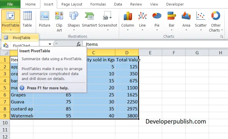
- Here, I have taken a set of fruits, their price, quantity sold, and their total value.
- Select the whole range, and click the Insert tab in the ribbon.
- Under the Insert tab, click Pivot tables and choose the destination for the pivot tables, either new sheet or Existing sheet.
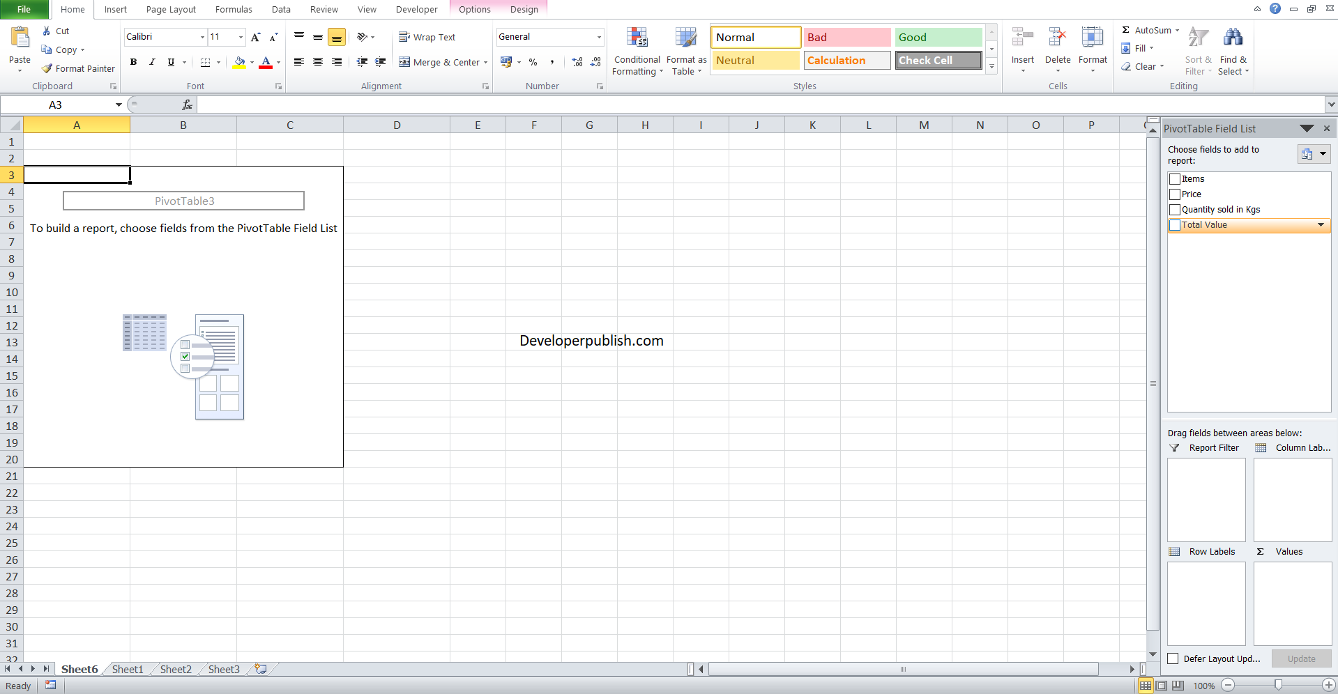
- When you choose a new sheet, the pivot table is inserted into a new worksheet.
- On the right side of your screen, you can find the field list pane.
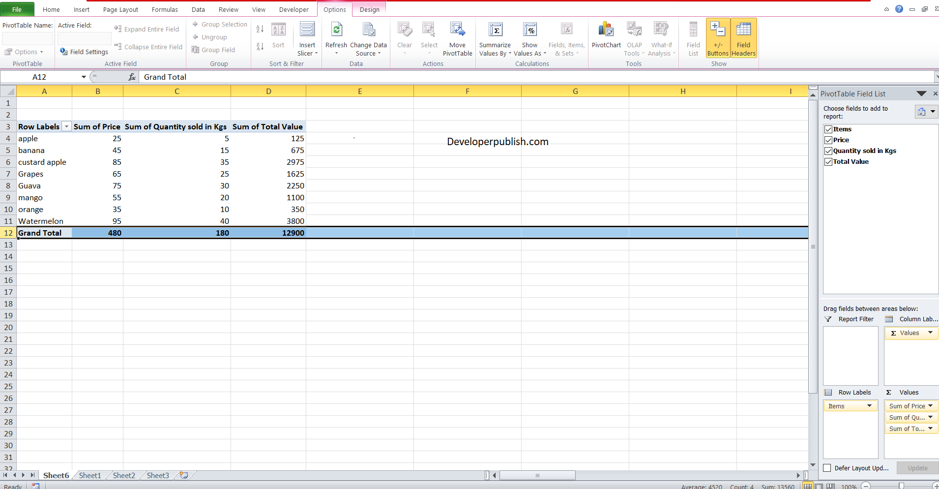
- Check the required fields and excel automatically sorts the fields in their places. (Row labels, column labels, etc.)
- You can see, Excel has created the grand total column on its own and it has summed up all the values in the respective rows.
- Now, let’s alter the pivot table.
- In the column labels, drag the ‘value’ to the row labels.

- The table gets altered and each item has its pricing and quantity in a group format.
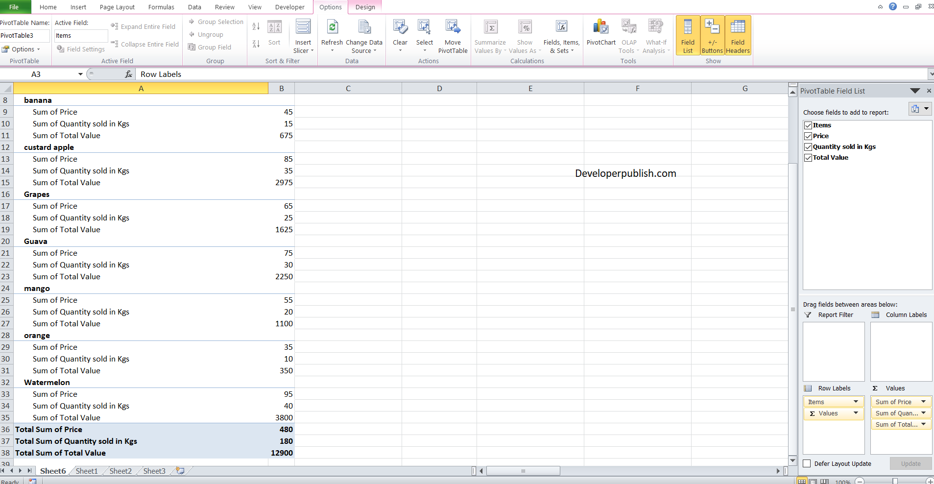
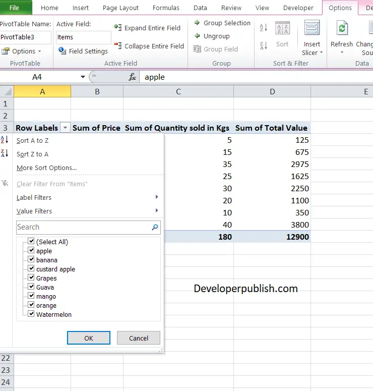
- By clicking the dropdown arrow in the row label, you can sort the items, add or remove items from the table.
How to Create PivotTable Manually?
- Select the cells for which you want to create a PivotTable.
- Click the Insert tab which in turn shows various Tables Group.
- From the Tables Group, select pivot table.
- A new dialog box opens, which shows the data selected by excel in default.
- From Choose the data that you want to analyze section, in Select a table or range, specify the range of the data.
- From the “Choose where you want the PivotTable report to be placed” section, select ‘New worksheet’ to place the PivotTable in a new worksheet or Existing worksheet, and then select the location you want the PivotTable to appear.
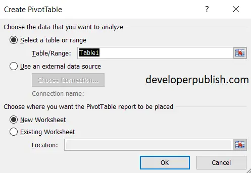
- Click OK
How to Format a PivotTable?
- Click anywhere in the PivotTable.
- PivotTable Tools tab appears on the ribbon.
- Under the Analyze or Options tab, in the PivotTable group, click Options.
- From the PivotTable Options dialog box, click the Layout & Format tab.
- You can format the table from the options.
How to Modify a Pivot Table?
- Click any cell in the pivot table.
- PivotTable Tools tab appears on the ribbon.
- Under the Options tab, in the PivotTable group, click the Field List button in the Show/Hide group.
- It displays the PivotTable Field List task pane.
- It shows the fields that are currently used in the table and its location that they’re currently assigned. You can modify them on your wish.
The following modifications can be made to the table’s fields:
Remove a field from the table
To remove a field from the table,
- You need to drag its field name from its current position into the sheet and release it when the mouse pointer changes to an x.
- Or else you can click its check box in the Choose Fields.
Move an existing field to a new place
To move an existing field to a new place,
- Drag its field name from its current label to a new label in the bottom of the task pane.
Add a field to the table
To add a field to the table,
- Drag the field name from the Choose Fields to Add to Report list and drop the field in the desired drop label.


