Filter in Excel works as a tool to show and hide the data in certain criteria. This post provides information about the Number and Text Filters in Excel.
Number Filter
The Number Filter in Excel helps us to filter only the numerical data. Let’s get to know how it exactly works.
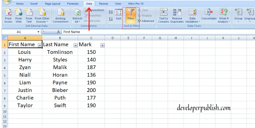
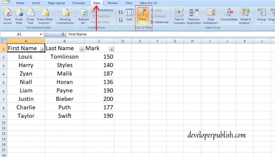
- After entering the required data place the cursor on any cell and go to the Data Tab. Click on the Filter icon, which you will notice in the data tab.
2. As soon as you click on the Filter option, you can see the Header arrow in each column. Click on the Header arrow and there will be a pop-up with a list of options.
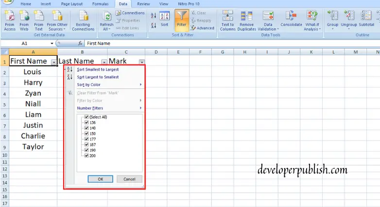
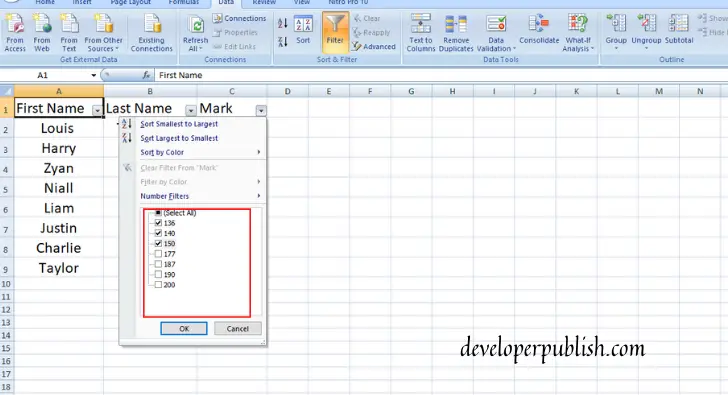
3. You can notice a list of pop-up, choose Number Filter option from that. Click on that and that will also give you a list of pop-up menus.
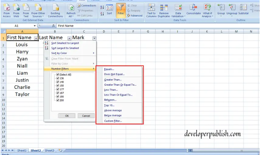
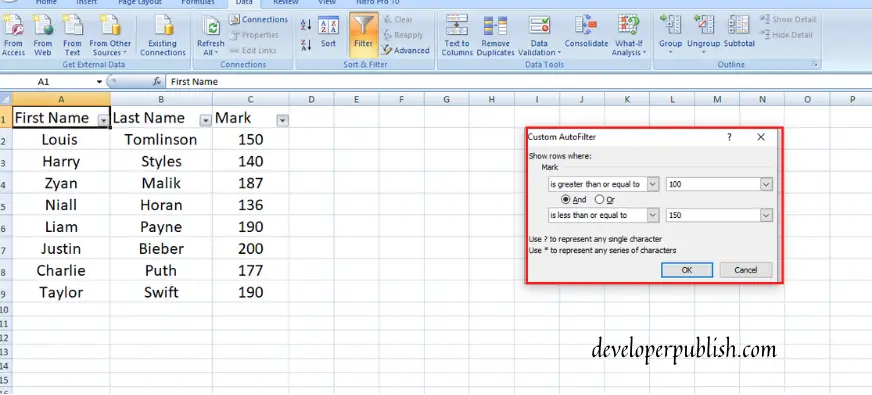
4. From that pop-up, you can choose either of the option to show the required and hide the rest. The Between option will take you to the custom filter dialogue box and from that, you can filter the data in either or pattern.
5. Or you can just uncheck the “Select all” from the pop-up and select the required & click ok.
This is how you can filter numerical data in excel. Let’s also know how to filter the text in excel.
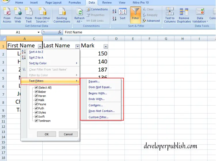
Text Filter
Text Filter is used to filter a set of data which is in text form. Filtering a text is as easy as the same way we filtered a numerical data.
- Place the cursor on a cell, click on the Data Tab and you will the Filter icon there. Click on that.
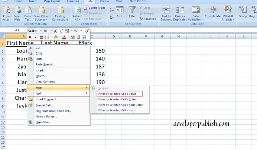
Or you can also use an easier way for filtering the data. Place the cursor on a cell, Right click on that cell and you will get a pop-up. Choose Filter option, this will also show a pop-up and choose Filter by cell value from those options.
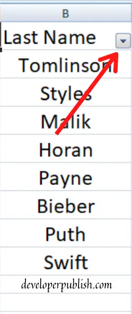
2. As soon as you click on the Filter option, each cell on the top of the column will get the Header arrow on it.
3. Click on the Header arrow, it will show a pop-up with a list of options. From those, choose Text Filter option which will again give a list of options.
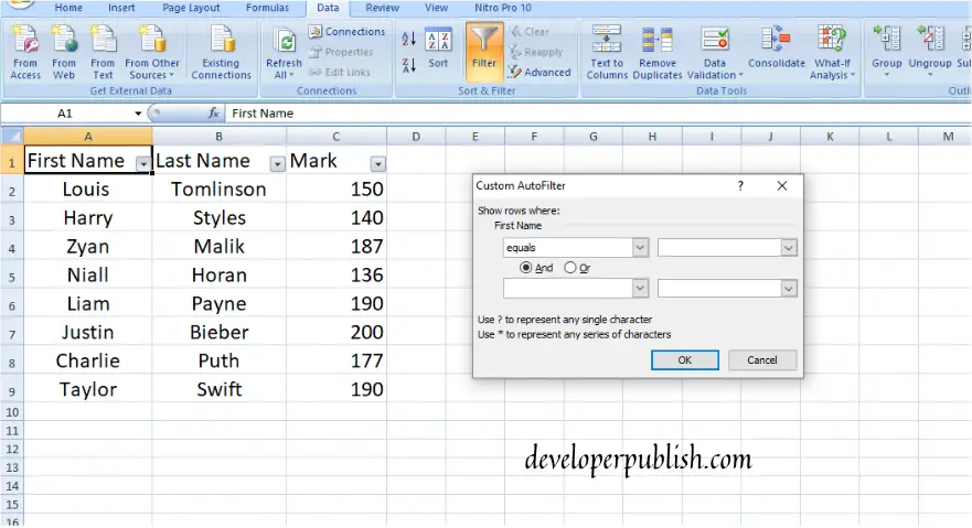
4.Choose either of the options listed in the pop-up. If you do so, it will show the custom sort dialogue box from which you can filter the text as you wish.
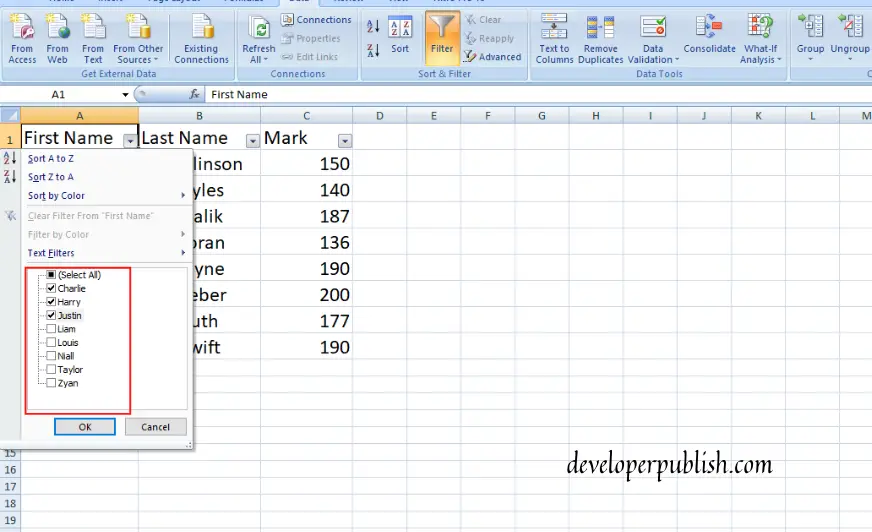
Or uncheck the Select all option and just select the names that have to be visible.
This is how a text or numerical data can be filtered in Excel. Hope this post was informative and gave the information you needed.


