In this post, you will be guided through simple and easy-to-follow steps to use the NPER function in Excel.
Microsoft Office Excel provides the NPER function, which returns the number of periods for loan or investment. In simpler words, the function helps to calculate the number of periods that are required to pay off a loan or reach an investment goal through regular periodic payments and at a fixed interest rate. It is a built – function in Excel categorized under Financial Functions.
NPER Syntax
=NPER(rate,pmt,pv,[fv],[type])
NPER arguments and functions
- rate (required) – The interest rate per period.
- pmt (required) – The payment made each period.
- pv (required) – The present value, or total value of all payments now.
- fv (optional) – The cash balance, or a future value you want after the last payment is made. (Defaults = 0)
- type (optional)– When payments are due. (Start of a period = 1, End of period = 0, Default = 0)
How to use the NPER function in Excel?
- Open Microsoft excel and launch a workbook or create a new Excel sheet.
- As said in the description, you need the values of all the above arguments to carry out the NPER function and get the correct and desired Number of periods.
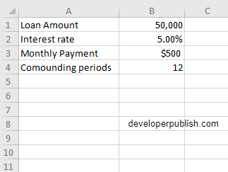
- Enter the arguments in the same order of the syntax, one below the other, in a similar way enter the values of each of the arguments in their corresponding adjacent cells in the worksheet as shown in the picture below.
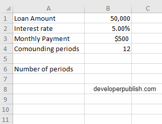
- Below the tabulated list of arguments, select a cell and enter “Number of periods”, the cell to the right will display the value of the formula (making identification easier).
- When entering the formula, always start with the “=” operator. After entering the “=” operator enter NPER to initiate the formula followed by an open parenthesis. Excel recognizes “=’ as the start of a formula, if not included, excel will not accept and evade the execution of the function.
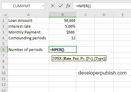
- With the parenthesis open, select the arguments in the order of syntax. The position of the cell will be visible in the formula. According to the order of the syntax, the value of the argument must be selected followed by a comma. The change in color of the cells aids to identify the name and of the cells in the formula.
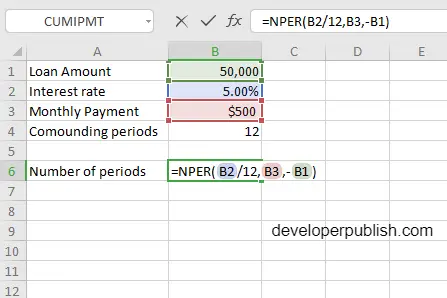
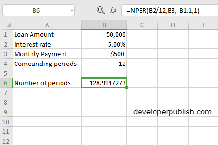
- Here, the payments are made monthly, so we needed to convert the annual interest rate of into a monthly rate by dividing the value by 12. The fv and type arguments are no included, where the value is considered as 0 by default.
- To conclude, close the parentheses and click enter. The cell which contains the formula will display the Number of periods.