Nested Fields in Excel PivotTable
In this post, you’ll learn about Nested fields in Excel Pivot table and how you can use it in your Excel worksheet.
Nested Fields in Excel PivotTable
When you have more than one field of data in an excel sheet, you can nest them or combine them into a meaningful cluster in the Pivot table which gives a meaningful report at the final stage. The PivotTable layout works depending on the order you place the fields in that area. This process is called nesting, and the fields in it are called nested fields.
Let’s understand the Nested fields’ concept in detail with the help of an example.
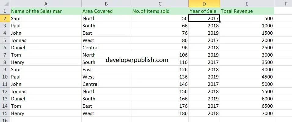
Take a look at the data given below:
It is a sales report of firm for the Year 2017-2019.
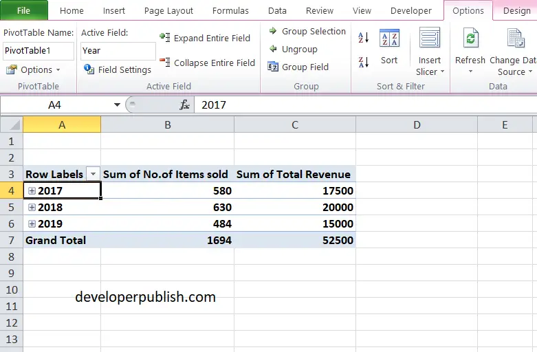
Now, let’s insert the pivot table in a new sheet.
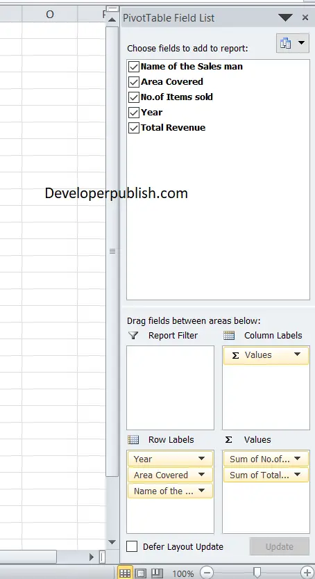
- From the field list, select the fields that you need for your report
- Drag and place them in your required area.
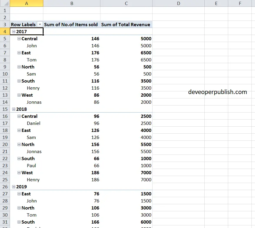
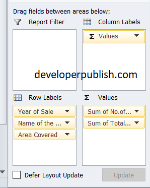
Here I have selected the Year of sale, Area Covered and Name of the salesman for the row field and the rest in the values field.
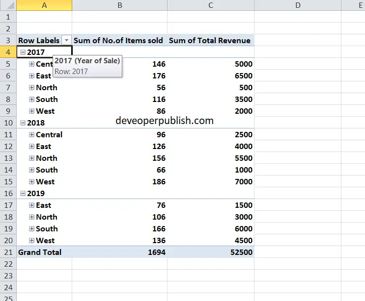
Now click on the ‘+’ icon near each Year of sale.
Areas covered during that Year of sale are listed inside the “Year of sale” field.
Click on the ‘+’ icon near the ‘Areas Covered’ and you can find the names of the Salesperson for each area during that particular Year of sale.
So the Name of the Sales person is nested inside the ‘Areas Covered field. And then the Areas Covered field is nested inside the “Year of sale” field.
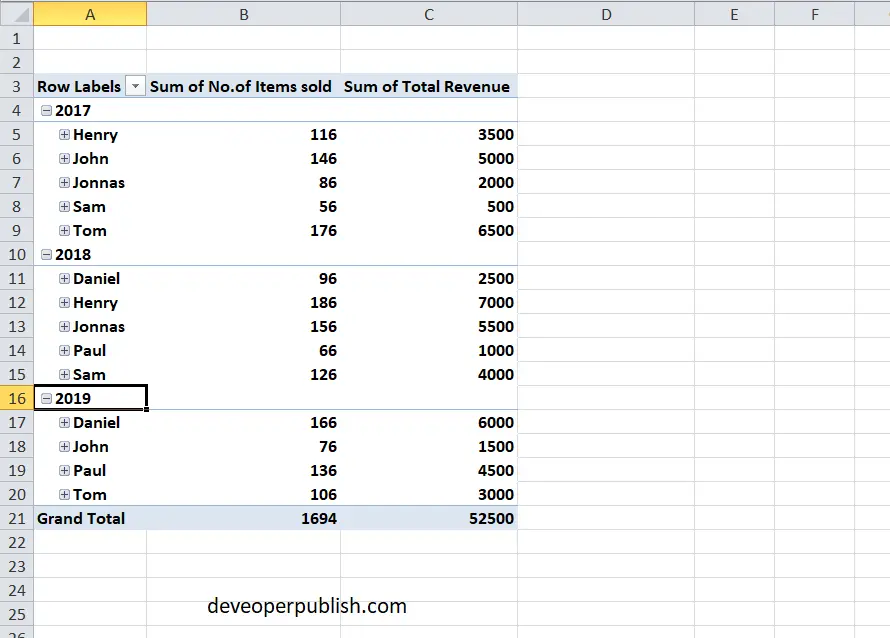
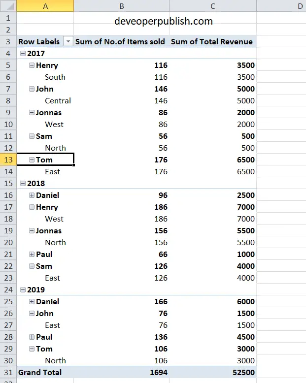
If we alter the position of row labels, then the report will change. For example, let’s move the ‘Name of the Sales person’ field between ‘Year of Sale’ and ‘Area Covered’.
Now the report looks like this.
When we click the year field, it shows the Name of the Sales persons working in that period of time.
And when click the sales person’s name, it then shows the area covered by them.
Therefore, when you understand your raw data, it is pretty easy to nest the fields inside other fields, making your report meaningful.



Leave a Review