In this post, you will be guided through simple and easy-to-follow steps on how to use the MIRR function in Excel.
Microsoft Office Excel provides the MIRR function, which returns the modified internal rate for a series of periodic cash flows. MIRR considers both the cost of the investment and the interest received on reinvestment of cash. This is a built-in Excel function under the Finance category.
MIRR Syntax
=MIRR(cash flows, financing_rate, reinvestment_rate)
MIRR function and arguments
- values (required) – Array or reference to cells that contain cash flows.
- finance_rate (required) – Required rate of return (discount rate) as percentage.
- reinvest_rate (required) – Interest rate received on cash flows reinvested as percentage.
How to use the MIRR function in Excel?
- Open Microsoft excel and launch a workbook or create a new Excel sheet.
- As said in the description, you need the values of the above arguments to carry out the IRR function and get the correct and internal rate.
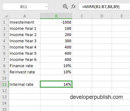
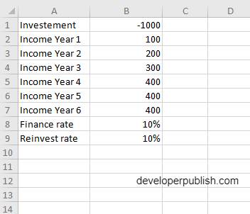
- Enter the arguments in the same order of the syntax, one below the other, as shown in the picture below.
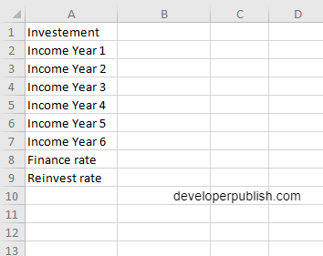
- At this time, in a similar way enter the values of each of the arguments in their corresponding adjacent cells in the worksheet.
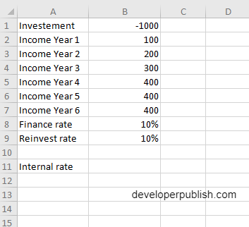
- Below the tabulated list of arguments, select a cell and enter “Internal rate”, the cell to the right will display the value of the formula (making identification easier).
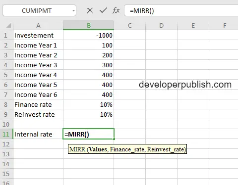
- When entering the formula, always start with the “=” operator. After entering the “=” operator enter MIRR to initiate the formula followed by an open parenthesis. Excel recognizes “=’ as the start of a formula, if not included, excel will not accept and evade the execution of the function.
- The initial investment here is a negative value as it is an outgoing payment, hence it can be enclosed in parentheses or given the negative sign. The cash inflows are represented by positive values.
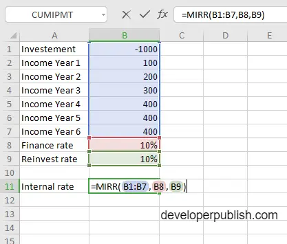
- With the parenthesis open, select the arguments in the order of syntax. The position of the cell will be visible in the formula. Here, as the argument values are entered in a group, use the fill handle to enter the values. The change in color of the cells aids to identify the name and of the cells in the formula.
- To conclude, close the parentheses and click enter. The cell which contains the formula will display the internal rate.