LCM Function in Excel
In this post you will lean about the LCM function, how to use in your excel spreadsheets.
LCM Function in Excel
The function returns the Least Common Multiple (LCM) of integers.
Syntax
=LCM(number 1, number 2,....)
The syntax initially has two arguments
- number 1 – This holds the first number
- number 2 – This holds the second number, default value 1.
The initial argument is required to perform the function whereas the next argument is optional as it has the default value 1.
How to use LCM Function in Excel?
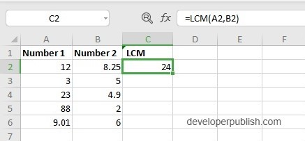
- The function returns the smallest multiple which is common between two number or more numbers. The functions work on integers and decimal numbers.
- For example:
- LCM(2,4) the answer is 8 as 8 is the smallest common multiple of 4 and 2 and LCM(3,4,5) the answer is 60 as 60 is the smallest common multiple of 3, 4 and 5.
- To start enter the numbers in the cells of the excel sheet
- In a new cell enter the syntax and highlight the cells to include them in the function.
- Press enter to display the answer.
- Use the fill handle to apply the function to the remaining data.
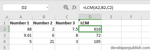
The examples below has more than 2 arguments
Additional Points:
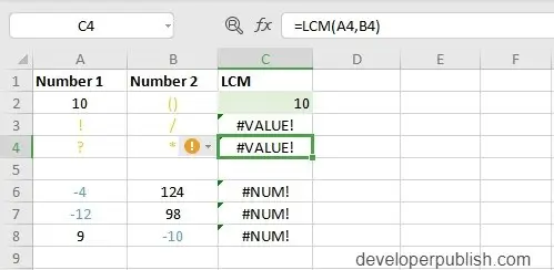
- The function does not accept non – numeric values and returns #VALUE!
- And similarly the syntax does not accept negative values, as a result it returns #NUM!
- The first row data does not show error as there is one value which can be accepted in the syntax.


Leave a Review