Inserting the color coded drop-down list in Microsoft Excel

There are times when you have to NOT just create or insert a drop-down list in Microsoft Excel sheet but also color code the value so that when the user selects a value from the drop down list , the color of the cell too changes.

How to insert color coded drop-down list in Excel 2016 ?

The conditional formatting in excel will help you to do it.

To begin with , we would need to create the drop-down list in Excel.

Create a drop down list in Excel

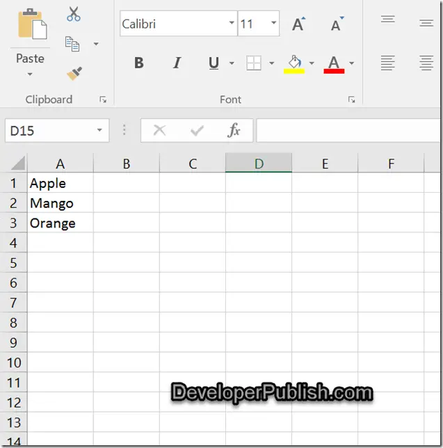
1. First , you need to create a list that you want the drop-down list to be populated with . So , let’s enter the values in the range A1 to A3 as shown.

3. Select the range of cells where you want the dropdown list to be inserted in to. In this example , lets select the cells C1 To C5.

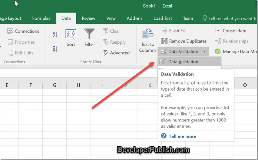
4. Click “Data –> Data Validation –> Data Validation” in Excel Ribbon.

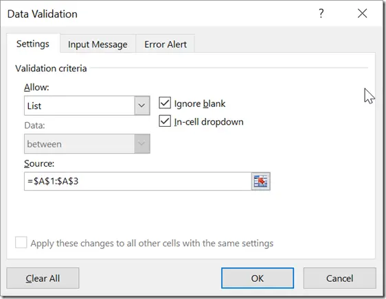
5. In the Data Validation dialog box , select the “Settings” tab and then choose the option “List” in the allow dropdown list and also select the list of values that you want to use as source. In his example , its A1 to A3.

6. Finally , Click the OK button to create the drop-down list. This should have inserted the drop-down list in the selected range of cells.

Add the Color code to the List in Excel worksheet.

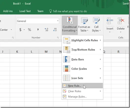
7. Further , highlight the drop-down cells . In this example , its C1 to C5 and the click “Home” –> Conditional Formatting –> New Rule.

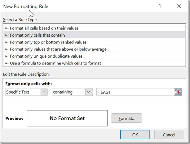
8. In the New Formatting Rule dialog , click “Format”” only cells that contain from the “Select a Rule Type” list box. Select “Specific Text” from the first dropdown list and containing from the 2nd drop-down list and specify the cell C1 in the textbox to specify that we are setting the color for the cell if the value is Apple.

9. Click on the Format button and choose the color that you to apply for this value. and then click the OK button. Perform the same steps for the other 2 values for the drop-down entries( for cells A2 and A3 as well.).

10. Finally , when you select the values in the cells C1 to C5 , you should see the corresponding colors that is set immediately …