How to Sort a Pivot Table in Excel?

In this post, you’ll learn how to sort a pivot table in your Excel spreadsheet.

Sort a Pivot Table in Excel

A pivot table in Excel allows you to sort the given data in ascending or descending order, which is very much useful in analyzing the data.

Let’s see an example.

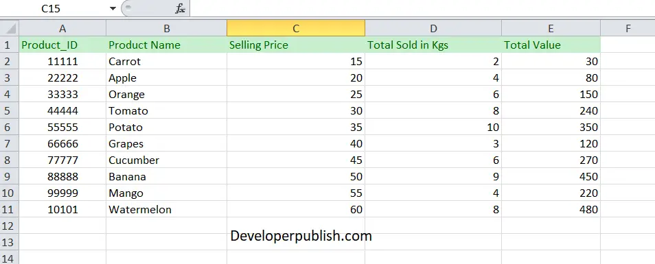
• Consider the following data.

• Select the range and under the Insert tab, click the pivot table option.
• Click the pivot table and insert it into a new worksheet.
• In the task pane, check all the fields which you feel necessary.

Now, let’s sort the pivot table.

You may see a drop-down arrow in the row and column fields. You can sort data either in row or column fields.

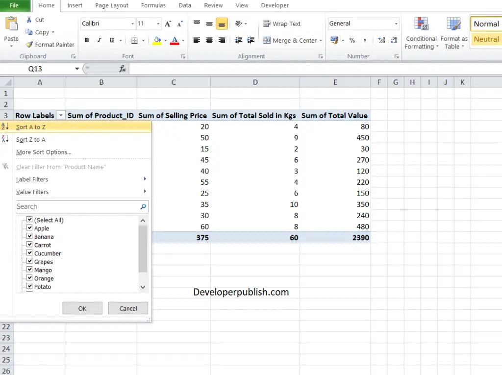
• Click the down arrow in the Row Labels.
• The drop-down menu contains the following options,

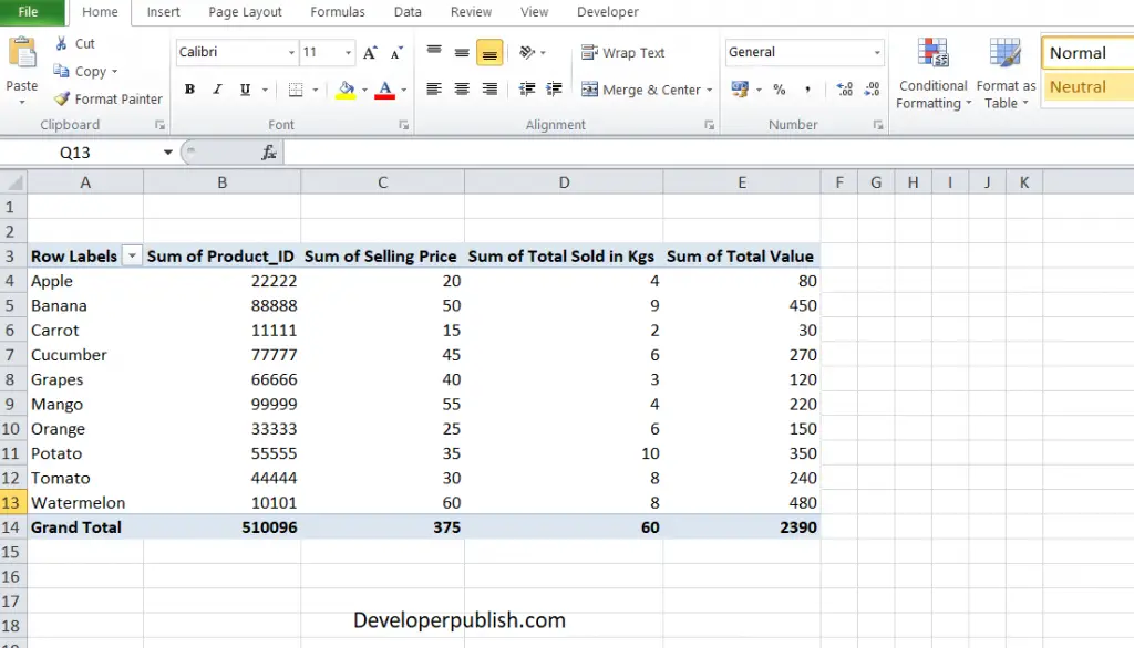
Sort A to Z: To sort the data from lowest to highest or in ascending order.

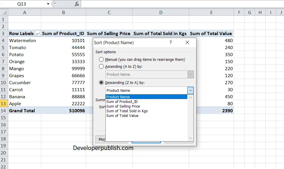
Sort Z to A:  To sort the data from highest to lowest order or in descending order.

More Sort Options:  This throws up another menu that has a manual sort option. You can sort the data on your own. Or you can choose the sort by option where you can command the pivot table to sort the given data based on the row or column labels.