In this post, you’ll will learn about Error Bars in Microsoft Excel and how to add error bars to a chart in Excel.
Error bars in Excel show the variability of data that we used in the chart. It basically helps to indicate the errors.
How to Add Error Bars to Chart in Excel?
To add the error bars to the chart in the worksheet, follow the below-mentioned steps:
- To get started, select the chart to add the error bars.
- Go to the Design Tab and click the Add Chart Elements option from the Charts Layout group.
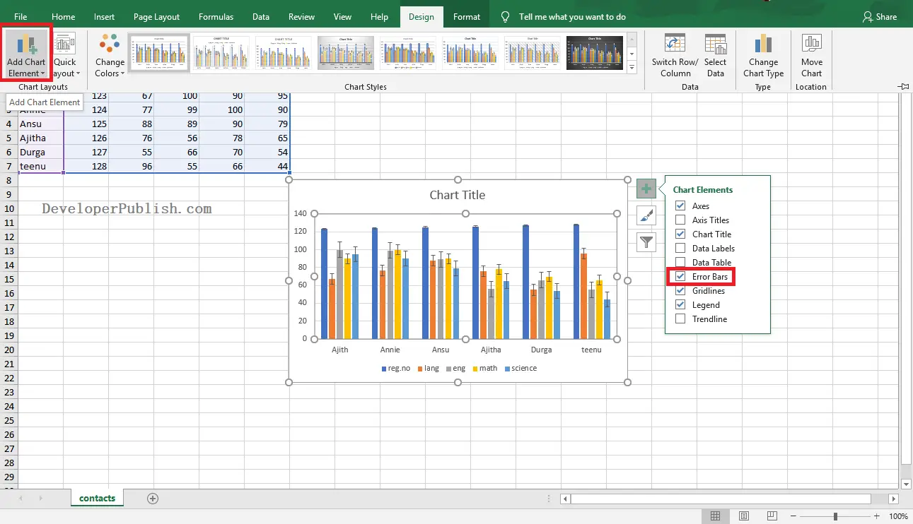
- Select the Error Bars option from the pop-down menu.
You can also get the Error Bars option by clicking the + symbol that appears at the top-right corner of the chart.
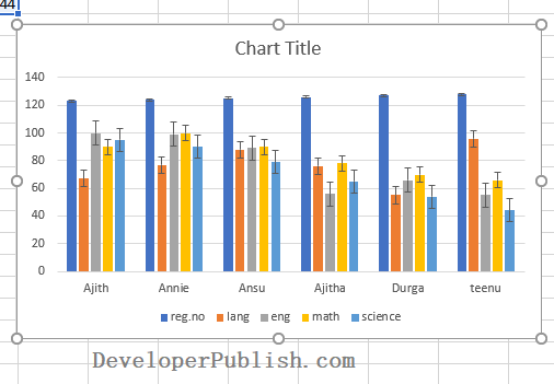
Now, you can see the added error bars as shown in the above image.