Formatting Values for Pivot Tables in Excel
In this post, you will how to format values for pivot tables in Microsoft Excel.
Formatting Values for Pivot Tables in Excel
When you place values into your Pivot Table, they won’t always be formatted how you want. Excel offers you a feature to format your values in the pivot table.
Let’s see it with an example.
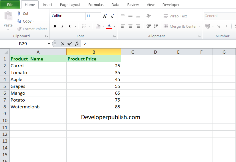
Look at the ex
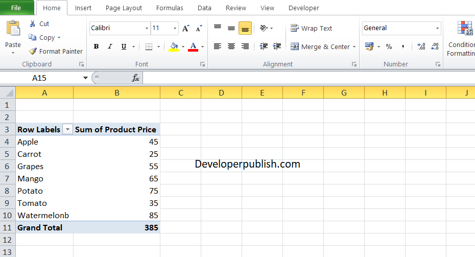
- Insert a pivot table for the data.
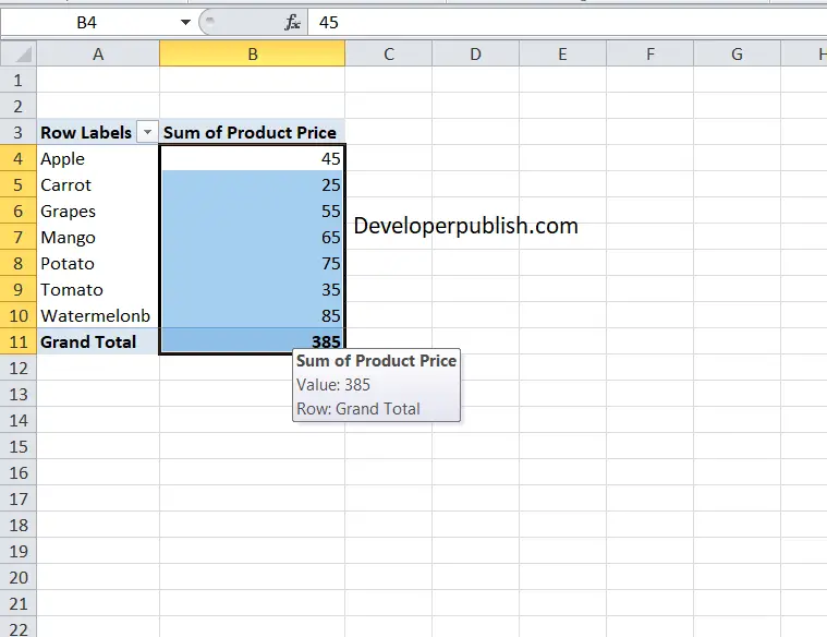
- Now, to format the values, Select the range of values that you need to format and right-click.
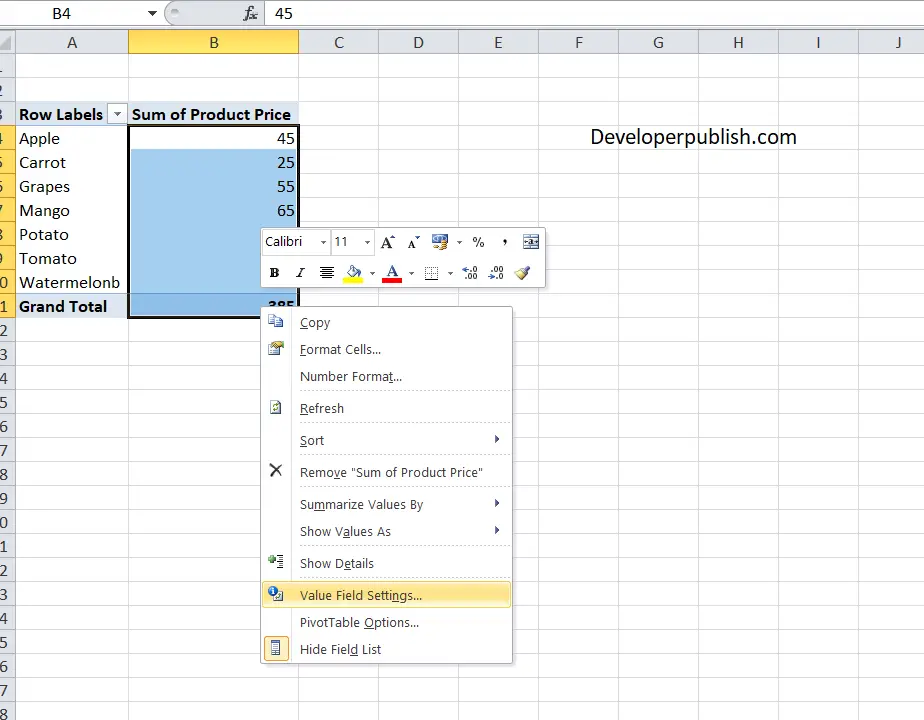
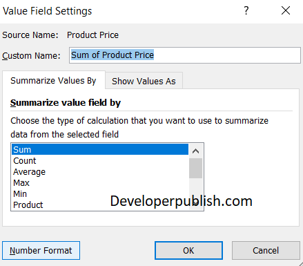
- Click on value field settings.
- The value field settings dialog box pops up. Click on the Number format on the bottom left corner.
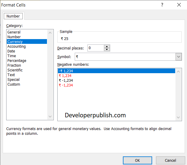
- In the format cell menu, under the number section choose the currency option.
- You can add decimal places to the value and you can also select the currency symbol.
Or
- Click the field drop-down menu in the field pane.
- Click Value field settings
- The value field settings dialog box pops up. Click on the Number format on the bottom left corner.
- In the Format cells dialog box, you can choose your formatting option.
Or
- Double click on the value field name.
- The value field settings dialog box opens and you can follow the same procedure to format your values.



Leave a Review