Dynamic Named Range in Microsoft Excel
This article is all about Dynamic Named Range in Microsoft Excel and how to use it in your excel workbook.
Dynamic Named Range is a feature in Microsoft Excel which automatically updates the data when changes are made in Named Range and only if the data is influenced by it or dependent on it.
How to implement a Dynamic Named Range in Microsoft Excel?
You’ll notice that the operation results you obtain based on Named Range remain the same even when the value in Named Range changes.
So to keep the worksheet updated follow the steps given below.
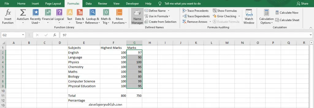
Select a Named Range.
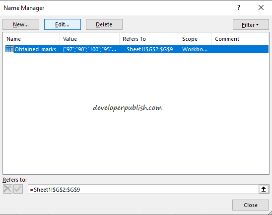
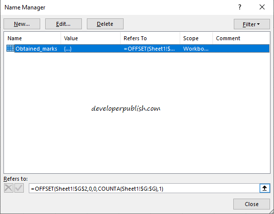
Go to Formula Bar in Menu Bar and select the Name Manager option in the Defined Names group.
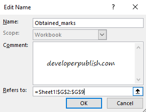
Select Edit in the Name Manager dialog box that opens up.
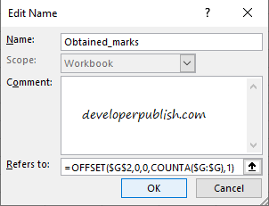
In the Refers to field add the OFFSET formula to expand the range.
OFFSET formula – OFFSET(first cell, 0, 0, COUNTA(column),1).
Here the first cell means the first cell of the particular row in the Named Range.
The 0, 0 refer to the rows and columns to offset. Since there no rows and columns to offset.
COUNTA function is used here to find the number of filled cells in the particular column. So when you add data to new cells it gets counted.
And the 1 is the width which equals to one column.
To proceed click on OK to implement it.
And then finally choose Close to save the changes.
The original data looks like this.
Now if you add data to new cells in the Named Range, the changes are reflected in the operations you’ve performed.
This is how you implement a Dynamic Named Range in Microsoft Excel.



Leave a Review