In this post, you will be guided through simple and easy-to-follow steps on how to use the COUPNUM function in Excel.
Microsoft Office Excel provides the COUPNUM function, which calculates the number of coupon payments that will be received, from the settlement date of the bond to its the maturity date, rounded up to the nearest whole coupon.
Table of Contents
COUPNUM Function in Excel
The COUPNUM function helps in returning the interest of payment or the number of coupons that is payable between the settlement date and the maturity date and is rounded up to the nearest whole coupon. This is a built-in function under the category Financial Function in Excel.
COUPNUM Syntax
=COUPNUM (settlement, maturity, frequency, [basis])
The COUPNUM function and arguments
- settlement (Required) – Settlement date of the security.
- maturity (Required) – Maturity date of the security.
- Frequency (Required) – Coupon payments per year (annual = 1, semi-annual = 2, quarterly = 4).
- Basis (Optional) – Day count basis (default =0).
How to use COUPNUM function in Excel?
- Open Microsoft excel and launch a workbook or create a new Excel sheet.
- As said in the description, you need the values of all the above arguments to carry out the COUPNUM function and get the correct and desired number of coupons.
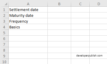
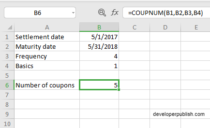
- Enter the arguments in the same order of the syntax, one below the other, as shown in the picture below.
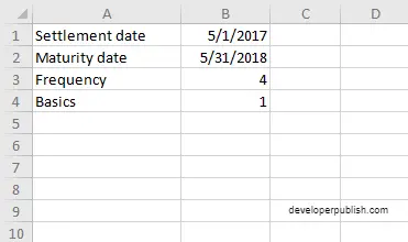
- At this time, in a similar way enter the values of each of the arguments in their corresponding adjacent cells in the worksheet.
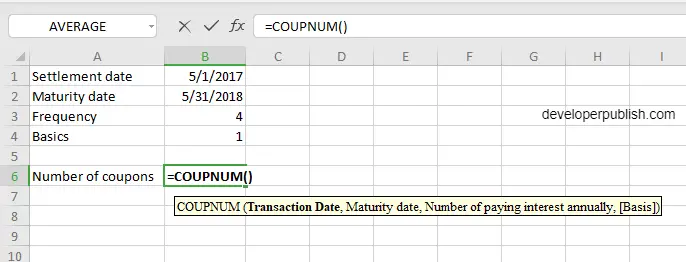
- Below the tabulated list of arguments, select a cell and enter “Number of coupons”, the cell to the right will display the value of the formula (making identification easier).

- When entering the formula, always start with the “=” operator. After entering the “=” operator enter COUPNUM to initiate the formula followed by an open parenthesis. Excel recognizes “=’ as the start of a formula, if not included, excel will not accept and evade the execution of the function.
- With the parenthesis open, select the first argument value. The position of the cell will be visible in the formula. According to the order of the syntax, the value of the argument must be selected followed by a comma. The change in color of the cells aids to identify the name and of the cells in the formula.
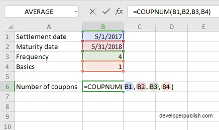
- To conclude, close the parentheses and click enter. The cell which contains the formula will display the number of coupons.
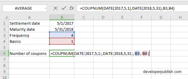
- Another method to carry out this function is by entering the date manually in the formula, followed by selecting the values for the last two arguments, where the position of the cell will be visible in the formula. It should be in this format COUPNUM(DATE(year,month,day),DATE(year,month,day),B3,B4)
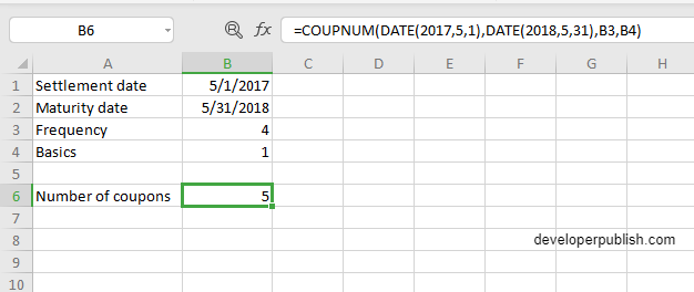
- Conclude the formula by giving the closing parenthesis, click enter. The cell which contains the formula will display the number of coupons.
.


