In this post, you’ll learn about what is AVERAGEA function in Microsoft Excel, its syntax and how to use AVERAGEA function in Excel spreadsheet.
What is an AVERAGEA function in Excel?
An AVERAGEA Function is used to calculate and return the AVERAGE(arithmetic mean) of a group of given numbers and text.
It differs from AVERAGE function as it include the logical value TRUE and FALSE, and numbers represented as text, whereas AVERAGE function just skips them during calculation.
AVERAGEA function is a built-in function which is also termed to be as statistical function. AVERAGEA Function is introduced in MS Excel 2007 and not available in older versions.
The AVERAGEA Function measures the central tendency(center of total numbers) in a statistical distribution.
The three most common measures of central tendency are:
- AVERAGE– which is used to calculate the arithmetic mean.
- MEDIAN-which is the middle number of the total number of values.
- MEAN-which is the frequently occurring number in the total number of values.
Syntax:
=AVERAGEA(value 1, [value 2]…,[value_n])
Parameters;
=> = – is a built-in function.
=> AVERAGEA () – is a functions name
=> value 1 -is a required argument(value).
=> [value 2] – is the second value(optional).
=>[value_n] – the total number of values.
Note:
- The values can be numbers, names, arrays, or references that contain numbers, text representation of numbers, logical values such as TRUE and FALSE.
- Empty cells, errors, and text are ignored.
- If you don’t want to include logical values and text , you can use AVERAGE Function instead of using AVERAGEA function.
Difference between AVERAGE function and AVERAGEA function
| AVERAGE FUNCTION | AVERAGEA FUNCTION |
| LOGICAL VALUES, LOGICAL VALUES WITH ARRAYS. They are counted as True =1, False =0, logical values with array are ignored. | They are counted as True=1, False =0, logical values with array are counted zeros. |
| TEXT Error value. | Error value. |
| EMPTY CELLS Ignored | Ignored |
How to use AVERAGEA Function in Microsoft Excel?
AVERGEA Function is a function which calculates the average(arithmetic mean) of the total number of given values.
Example:
In AVERAGEA function we can use logical values, name and numbers.
Step 1:
- Open the workbook in the Microsoft Excel. Now enter a logical function TRUE in A1 and select the cell where you want to calculate the value.
- In the selected cell enter ‘= AVERAGEA’ and open the parenthesis, enter the row name A1 and close the parenthesis.
- Then press ENTER to calculate the result.
- The result will be 1 for true, since the value of true is 1.

Step 2:
- Open the workbook in the Microsoft Excel. Now enter a logical function FALSE in A2 and select the cell where you want to calculate the value.
- In the selected cell enter ‘= AVERAGEA’ and open the parenthesis, enter the row name A2 and close the parenthesis.
- Now press ENTER to calculate the result.
- The result will be 0 for false, since the value of false is 0.

Step 3:
- Now enter a name in A3 and select the cell where you want to calculate the value.
- In the selected cell enter ‘= AVERAGEA’ and open the parenthesis, enter the row name A3 and close the parenthesis.
- Now press ENTER to calculate the result.
- The result will be 0.

Step 4:
- Now we enter numbers in A4 and A5, select the cell where you want to calculate the value.
- In the selected cell enter ‘= AVERAGEA’ and open the parenthesis, enter the row name A4 And A5 and close the parenthesis.
- Now press ENTER to calculate the result.
- The result will be the same numbers.
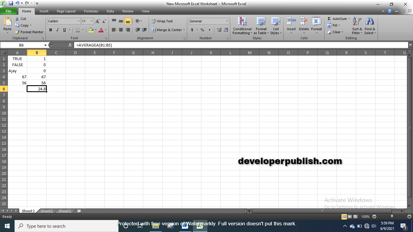
Step 5:
- Now we calculate the total number of given values. Select the cell where you want to calculate the value
- In the selected cell enter ‘= AVERAGEA’ and open the parenthesis, enter the row name as A1:A5 and close the parenthesis.
- Now press ENTER to calculate the result.
- The example is shown in the above screenshot.


