Selecting, Moving, & Clearing Pivot Table Data in Excel
In this post, you’ll learn the basics of selecting, moving, and clearing pivot table data in Excel.
Selecting, Moving, and Clearing Pivot Data in Excel
There are circumstances when you need to alter multiple fields are select the whole pivot table and perform actions like moving it to a new worksheet or copying the table and pasting it somewhere on the existing sheet or maybe clearing the filters or the table, you can perform all these actions by selecting few options rather than performing it manually.
Let’s us learn how to select the pivot table.
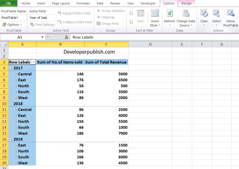
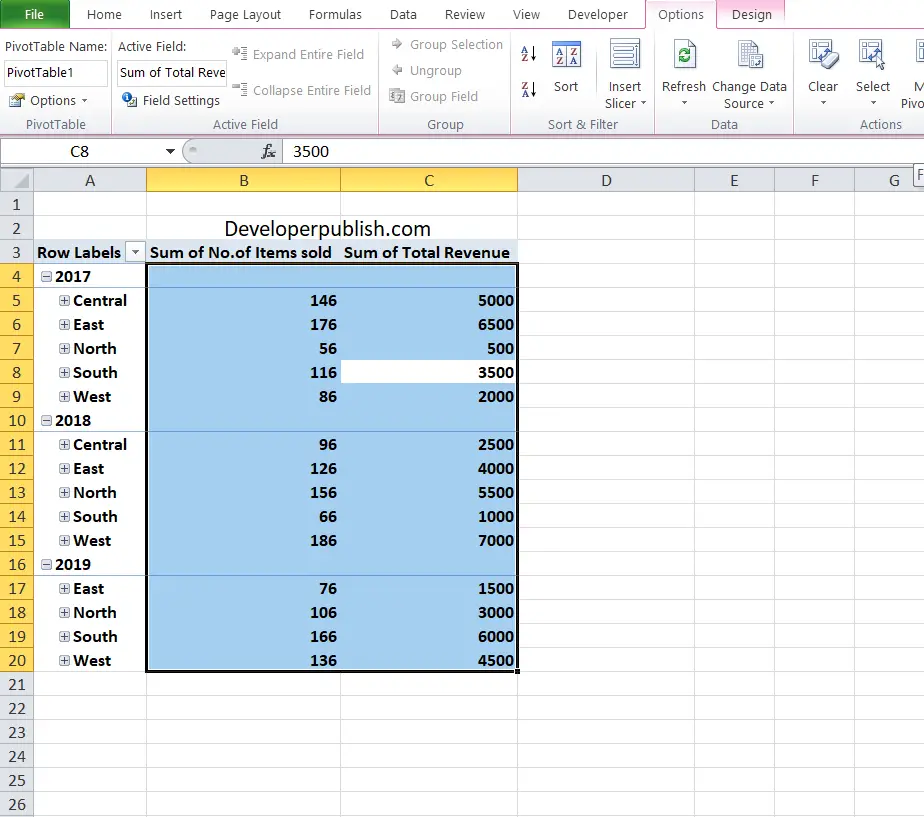
Take a look at the example.
Selecting the Pivot table
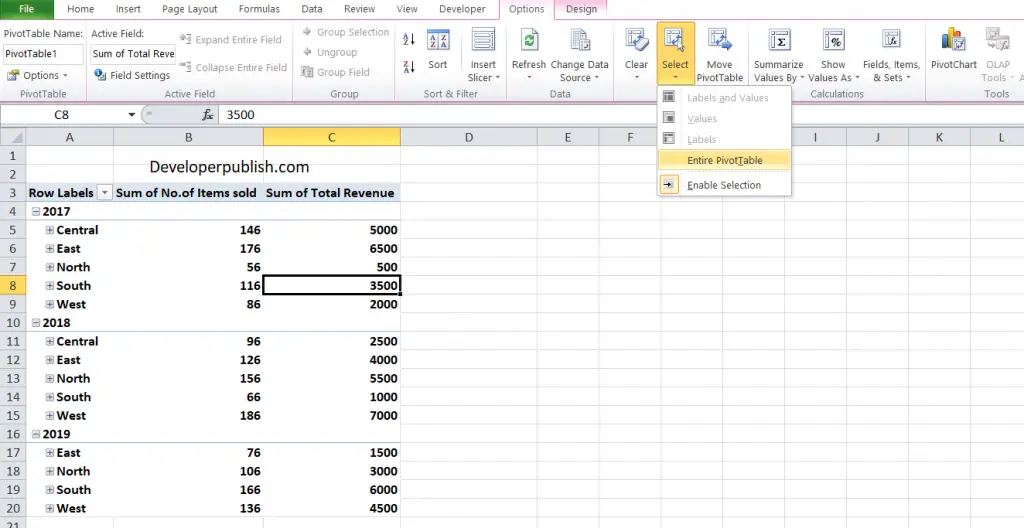
To select the pivot table, Click on any cell in the pivot table.
In the options tab in the ribbon, click the select icon.
From the dropdown, select the option “Entire Pivot Table”.
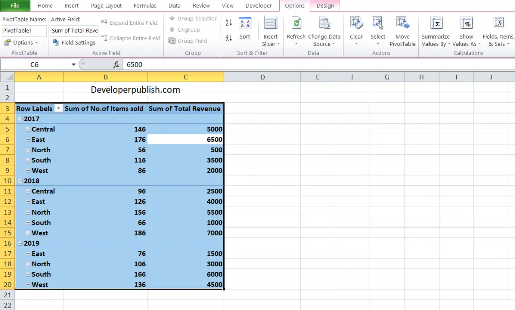
The whole pivot table gets selected.
By selecting this feature, the other options like, Labels, values and labels and values are enabled.
Labels: This option selects only the labels of the Pivot table
Values: This option selects only the values present in the Pivot Table.
Moving the Pivot Table
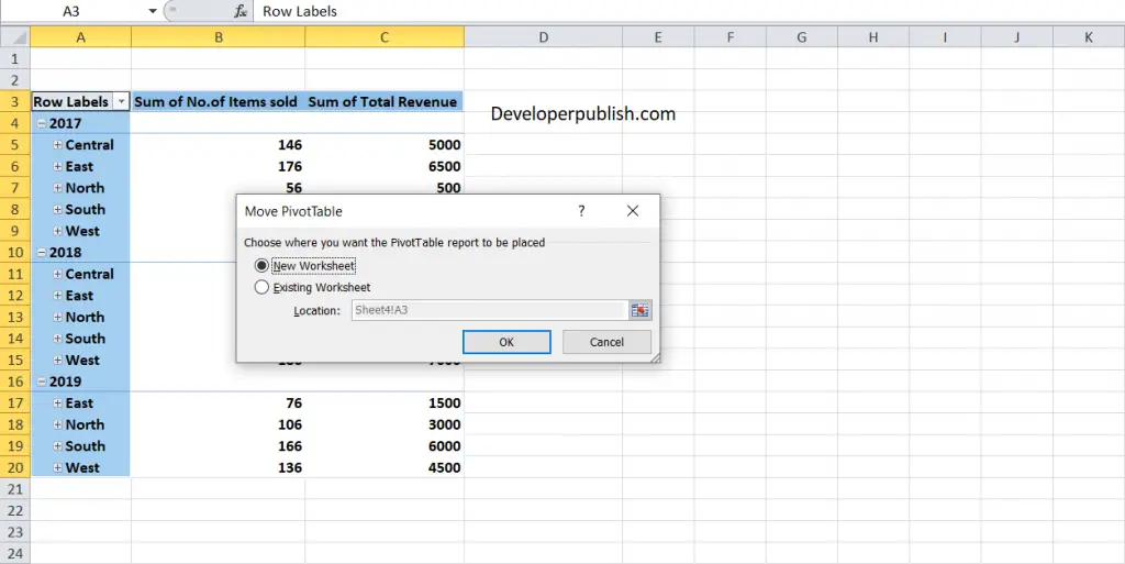
In the same Options tab ribbon; you can see the icon “Move Pivot Table”.
Click on it and the Move pivot table dialog menu opens, you can choose to move the pivot table to new worksheet or Existing worksheet along with the location of the table.
Clearing the Pivot Table
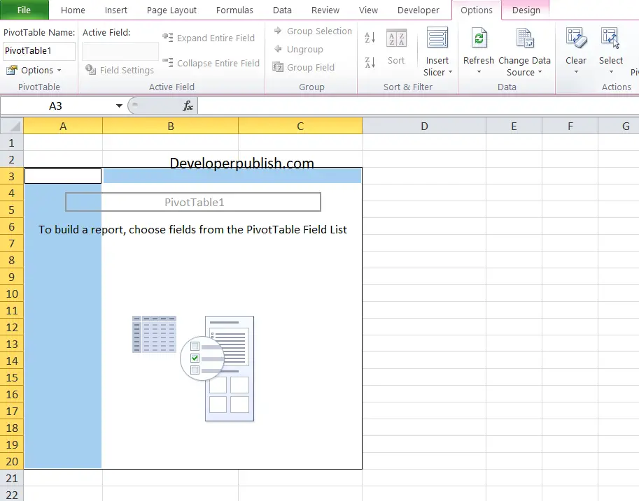
The clear icon in the options tab has a drop down menu.

Using this you can clear the entire pivot table or the filters applied to the Pivot table.
The clear operation is completely different from deleting a Pivot table. It does not delete the data, just allow you to start over once again.
This option is very much useful, at times when we mess up with our labels and fields.




Leave a Review