RANK Function in Excel

In this article, you will learn about the RANK function, the formula syntax, and usage of the function in Microsoft Excel.

RANK Function in Excel

The RANK function in Excel returns the rank of a numeric value when compared to a list of other numeric values. RANK can rank values from largest to smallest as well as smallest to largest.

Important: Excel has replaced this function with one or more new functions to improve accuracy along with the function names reflecting their usage. But still, the function is still available for backward compatibility, you should consider using the new functions like RANK.AVG function and RANK.EQ function because this function may not be available in future versions of Excel. 

Syntax

=RANK(number,ref,[order])

Arguments:

• Number    – The number whose rank you want to find.
• Ref    – An array of, or a reference to, a list of numbers. Non-numeric values in ref are ignored.
• Order –  A number specifying how to rank a number. (Optional)

Usage Notes and Possible Errors

• When the order is 0 or omitted, Excel by default ranks the number as if ref were a list sorted in descending order.
• When the order is any nonzero value, Excel by default ranks the number as if ref were a list sorted in ascending order.

• The RANK function gives duplicate numbers the same rank.
• Correction factor for tied ranks=[COUNT(ref) + 1 – RANK(number, ref, 0) – RANK(number, ref, 1)]/2.

How to use the RANK function in Excel?

Using this function in a WS is simple; all you need to do is enter the function as a formula of the cell in the formula bar.

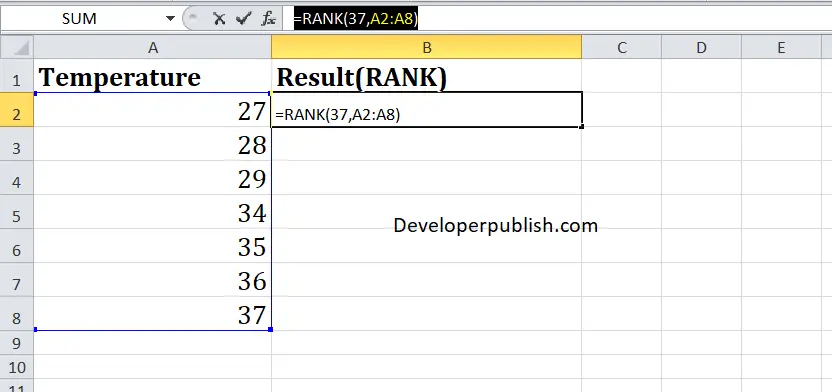
Take a look at the given example

Enter the data in the respective columns and enter the RANKfunction formula.

Formula: =RANK(37,A2:A8)

Here, A2 refers to the cell name or the cell address. Column A denotes the Array.