QUARTILE Function in Excel
In this article, you will learn about the QUARTILE function, the formula syntax and usage of the function in Microsoft Excel.
QUARTILE Function in Excel
The QUARTILE function in Excel returns the quartile for a given set of data. Using the QUARTILE function, you can get the minimum value, first quartile, second quartile, third quartile, and max value.
Note: Excel has replaced this function with one or more new functions to improve accuracy along with the function names reflecting their usage. But still, the function is still available for backward compatibility, you should consider using the new functions like QUARTILE.EXC function and QUARTILE.INC function because this function may not be available in future versions of Excel.
Syntax
= QUARTILE(array, quart)
Arguments:
- Array – The array or cell range of numeric values
- Quart – Indicates which value to return
| Quart Value | QUARTILE returns |
| 0 | Minimum Value |
| 1 | The first quartile (25th percentile) |
| 2 | Median value (50th percentile) |
| 3 | Third quartile (75th percentile) |
| 4 | Maximum value |
Usage Notes and Possible Errors
- When an array is empty, the QUARTILE function returns the #NUM! Error value.
- The quart value is truncated.
- When the quart < 0 or if quart > 4, the QUARTILE function returns the #NUM! error value.
- MIN, MEDIAN, and MAX return the same value as QUARTILE when quart is equal to 0 (zero), 2, and 4, respectively.
How to use the QUARTILE function in Excel?
Using this function in a worksheet is simple; all you need to do is enter the function as a formula of the cell in the formula bar.
Take a look at the given example

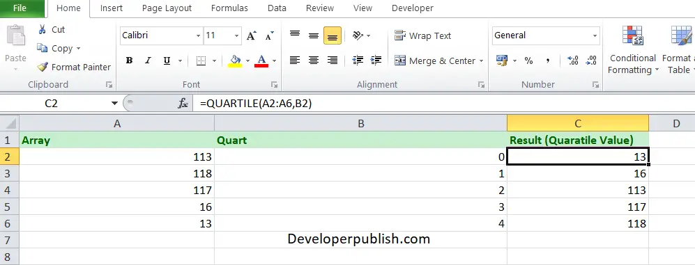
Enter the data in the respective columns and enter the QUARTILE function formula.
Formula: =QUARTILE(A2:A6, B2)
Here, A2 refers to the cell name or the cell address. Column A denotes the Array and Column B denotes the quart value. Here, we have shown all the quart values from 0-4.
You will get the result in the Result column.


Leave a Review