How to highlight alternate rows or columns in Microsoft Excel 2016 using conditional formatting feature?
There are various ways in which you can color the alternate rows or column in excel and these include the conditional formatting and table designs.
This blog post will demonstrate how to automatically highlight alternate rows or columns in Microsoft Excel 2016 using the Conditional formatting feature.
How to highlight alternate rows or columns in Microsoft Excel 2016 using conditional formatting feature?
1. Launch Microsoft Excel 2016 and open your worksheet that contains the data.
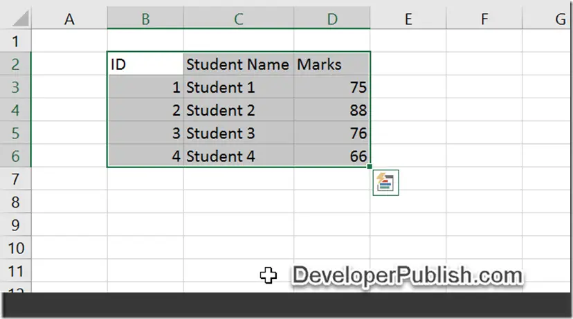
2. Select the rows that you wish to highlight or apply shades using the conditional formatting.
3. Now , navigate to the “Home” ribbon and then click on the “Conditional Formatting” dropdown list and select “new rule”.
4. In the “New Formatting Rule” dialog , select “Use a formula to determine which cells to format” from the “Select a Rule Type” list box and then enter the formula =mod(row(),2)=0 in the “Format values where this formula is true” textbox.
5. Click the “Format” button. In the Format Cells Dialog , select the Fill tab and then set the background color. In this example , let me select Blue and click OK button.
6. You will see that the alternate rows are highlighted for the selected data.
You can use the formula =MOD(COLUMN(),2)=0 for highlighting alternate columns in Microsoft Excel 2016 by following the same steps as defined in this blog post.


Leave a Review