In one of the previous blog posts , I explained how the users can use the conditional formatting feature in Microsoft Excel 2016 to highlight alternate rows or columns.

In this blog post , let’s explore the table style feature to highlight alternate rows or columns in excel.

How to highlight alternate rows or columns in Microsoft Excel 2016 using Table Style?

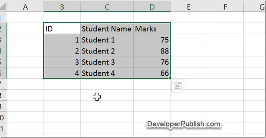
1. Open the workbook in Microsoft Excel 2016 and then select the cells that needs to be formatted.

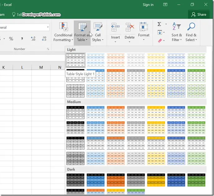
2. Click on the the “Format as Table” dropdown box and select any table format that you like.

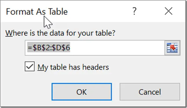
3. This will display the “Format As Table” dialog. If you already have a header in the selected cells , enable the checkbox “My table has headers” and click OK button.

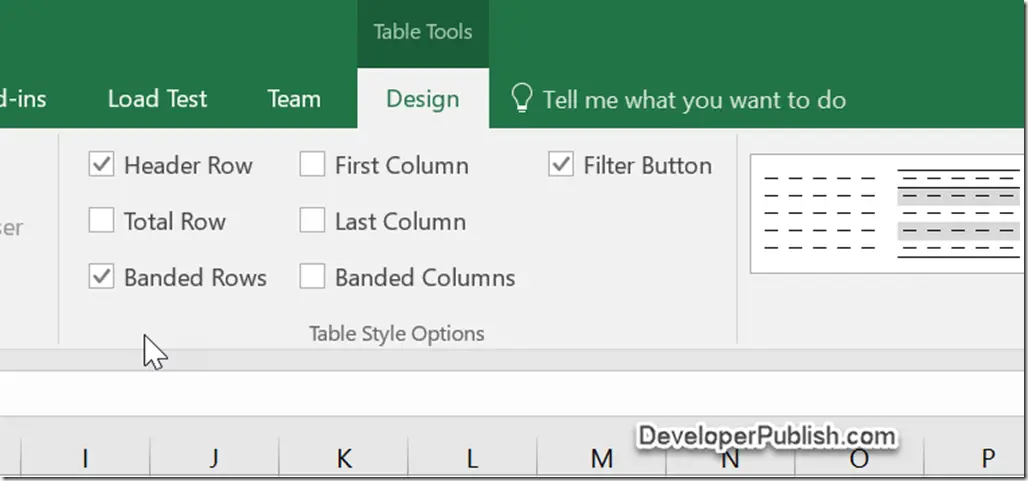
4. With the data selected , you should now see a new tab called “Design” which would be selected and displays additional options. Select the checkbox “Branded Rows” to highlight alternate rows. The Branded Column checkbox can be used to highlight alternate columns.

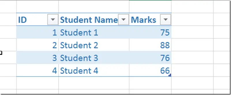
You should see the data with the alternate rows highlighted…