CEILING Function in Excel
In this post, you will learn about a very simple function in Excel – Ceiling Function and how to use it with-in excel spreadsheet.
CEILING Function in Excel
The Ceiling function rounds up a given number to the nearest specified multiple. This function always rounds up the number to the next higher value, and so the name Ceiling.
Syntax
=CEILING(number, significance)
Parameters
The syntax has the following arguments
number – The number that you want to round up; Required
significance – The multiple to which you want to round the number; Required
- The Ceiling function rounds up the given number to the closest multiple of the significance value.
- Both the arguments in the syntax can be an integer or decimal number.
- Note that the number is rounded up according to the multiples and not the number itself Example =CEILING(10, 3) answer is 12 a multiple of 3 .
- Sometimes when the significance value is 1, the function returns the number unchanged as the answer. This happens when there is no need to round up the number as it satisfies the significance value.
Examples of the Ceiling Function
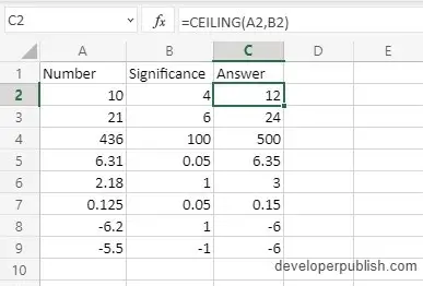
In the above example, both the arguments are displayed and inserted in the syntax.
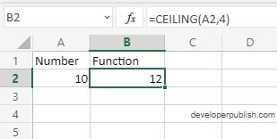
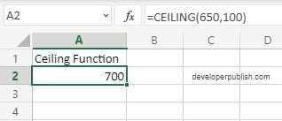
You can also enter the arguments in the Ceiling function syntax , like the following examples.
Additional notes
- #VALUE! – when any one the arguments has a non numeric value.
- When rounding up a negative number:
- If the significance value is positive the answer is rounded up, moving towards zero.
- In negative numbers -6 is greater than -6.2, so when we round up the number with a positive significance value the answer is greater.
- In then same way when the significance value is negative the value is rounded down, moving away from zero.
- Here -6 is lesser than 5.5, so when we round up the number with a positive significance value the answer is lesser.


Leave a Review