BIN2OCT Function in Excel
In this article, you will learn about the BIN2OCT function, its usage, syntax, and how to use it in your excel spreadsheet.
BIN2OCT Function in Excel
The BIN2OCT function in Excel converts a binary number to its octal values.
Similar to the BIN2DEC and BIN2OCT, the input numbers must contain only zeros and ones and restricted to only ten characters, and if the value crosses the ten character limit, the function will return “#NUM!” Error.
Syntax
= BIN2OCT(number, [places])
Arguments:
- Number – The binary number that you wish to convert.
- Places [optional] when left out or neglected, it uses the least number of characters required to represent the number, or else it combines the result with zeros up to the specified number of places.
Possible Errors
- When the entered number is Not a valid binary number, or the number contains more than 10 characters (10 bits), BIN2OCT returns the #NUM! error value.
- And when the entered number is negative, BIN2OCT ignores places and returns a 10-character octal number.
- When BIN2OCT requires more than ‘places’ characters, it returns the #NUM! error value.
- And when the ‘places’ is not an integer, it will be truncated.
- When the ‘places’ is non-numeric, BIN2OCT returns the #VALUE! error value.
- When the ‘places’ is negative, BIN2OCT returns the #NUM! error value.
How to use the BIN2OCT in excel worksheet?
Using this function in a WS is simple; all you need to do is enter the function as a formula of the cell in the formula bar.
Take a look at the given example
Binary numbers:
- 10100010
- 100101
- 1000100
- 101010
- 100101001
- 10101010010
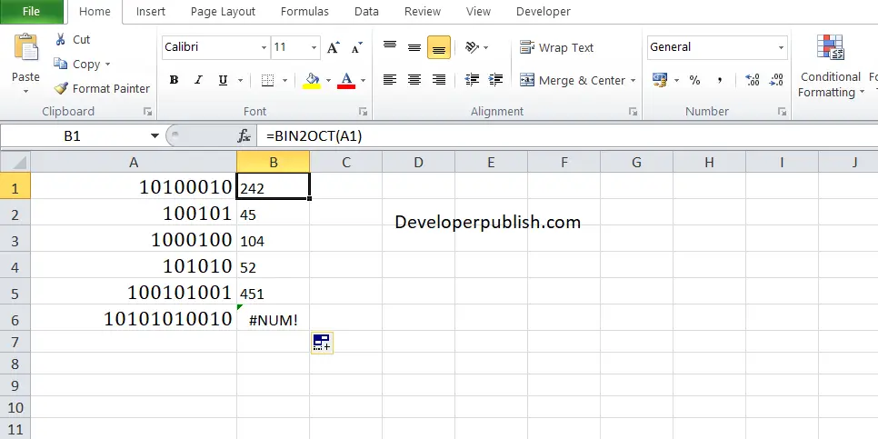
The above numbers are the binary version of some Octal numbers. To find out the Octal numbers, Enter the given binary numbers in column A and in Column B, enter the following formula
Formula: =BIN2OCT(A1)
Here, A1 refers to the cell name or the cell address. Repeat the same to the other cells and you will get the Octal value of the binary values.

In Cell A6, you can find that the corresponding value is #NUM! error, that is due to the presence of more characters than the prescribed limit of 10.


Leave a Review