This post is about the Vlookup feature and its various options in Microsoft Excel and how you can use it effectively to improve your productivity when using Excel.
Vlookup in Microsoft Excel
The VLOOKUP (i.e Vertical Lookup) function finds for a value in the leftmost column of a table and then displays the value in the same row from another column you specify.
Syntax:
VLOOKUP(lookup_value, table_array, col_index_num, [range_lookup])
Vlookup – Exact Match in Excel
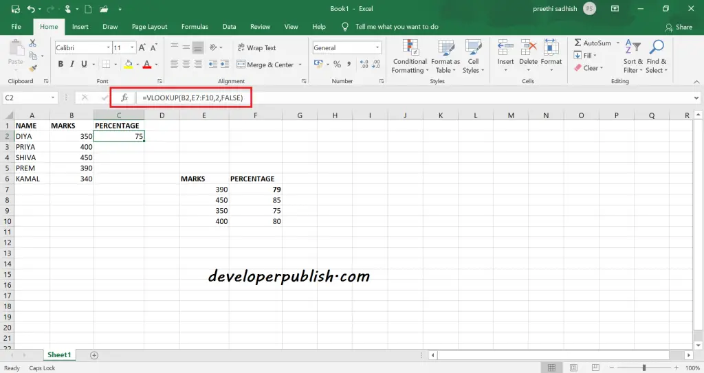
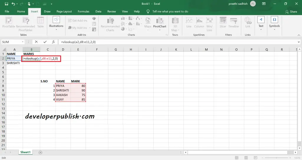
Using Vlookup you can find an exact match, by setting the 4th argument (i.e range-lookup) to FALSE or zero.
=VLOOKUP(value, data, column, False)
=VLOOKUP(value, data, column, 0)
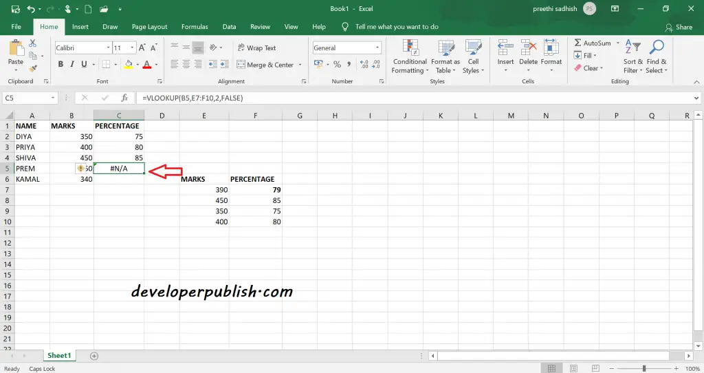
If the Vlookup can’t find an exact match then it returns #N/A.
Vlookup – Approximate Match in Excel
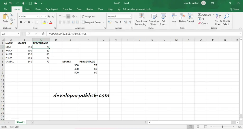
To find an approximate match using Vlookup then set the 4th argument (i.e range-lookup) to TRUE or 1 or omit the 4th argument.
=VLOOKUP(value, data, column, True)
=VLOOKUP(value, data, column, 1)
Vlookup – Looks Right in Excel
What are the Limitation of Vlookup ?.
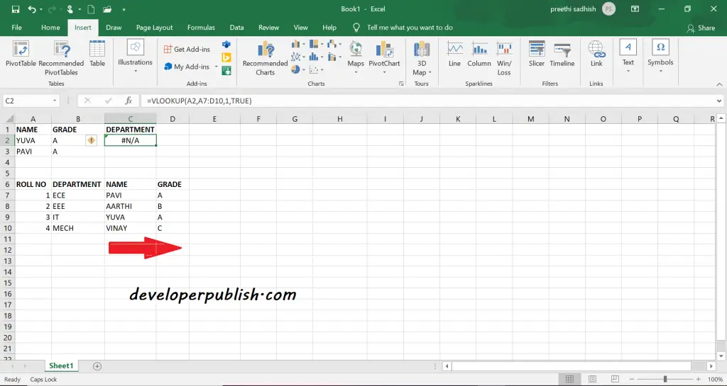
Vlookup can only look to the right to retrieve data.
This means that the function searches for the value only to the right side of the lookup_value.
In these cases, Index and Match can be used.
Here using the name as lookup value you can only find the values to the right of the lookup value. Hence you can only get the grade but not the department.
Vlookup – First Match in Excel
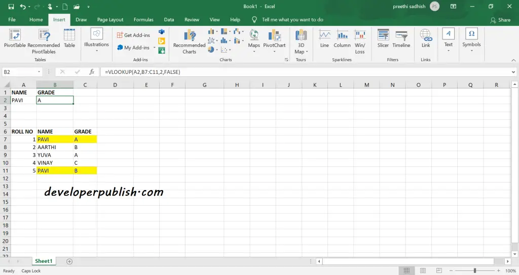
If a lookup_column contains duplicate values, Vlookup will match the first value only.
Vlookup – Case insensitive in Excel
Vlookup takes both upper and lower case as the same. So it is case insensitive.
Vlookup – Multiple criteria in Excel
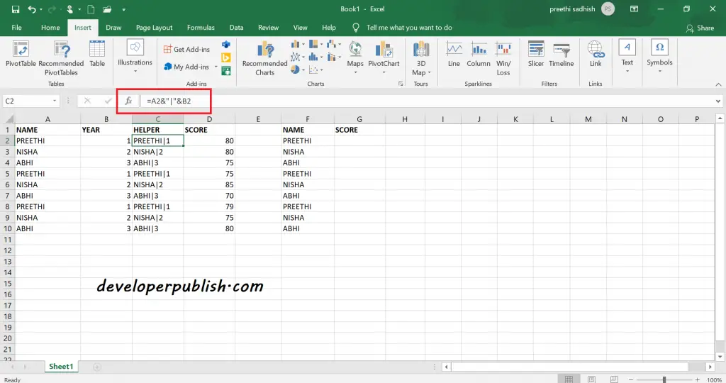
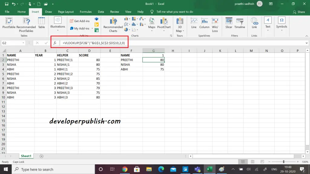
Generally, the Vlookup function cannot handle multiple criteria. In this case you can use a helper column to join multiple fields together and then use this field inside a Vlookup function.
=VLOOKUP(val1&val2, data, column, 0)
Here the helper column is the concatenation of name and the year. Now, with the reference of this column you can get the score of 1st year alone using VLOOKUP function.
#N/A Error in Excel
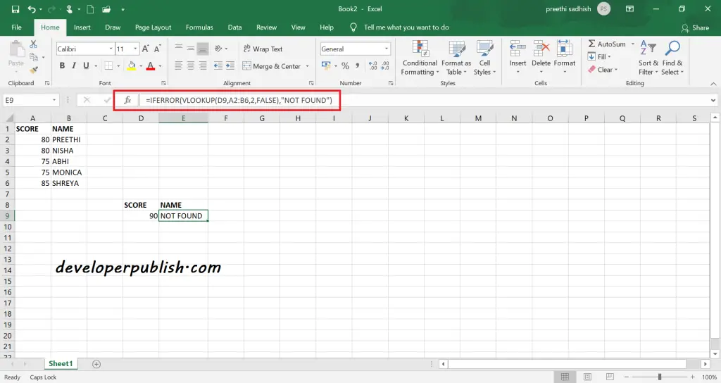
VLOOKUP will display the #N/A error when no match is found in the exact mode. Instead of #N/A, you can display a meaningful message. This can be done by using the IFERROR function with the Vlookup function.
=IFERROR(VLOOKUP(lookup_value, range, column_index, range_lookup),”Not found”)
Vlookup – Multiple Lookup Tables in Excel
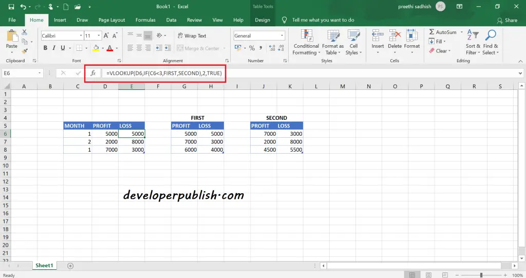
To lookup value from multiple tables, the Vlookup function is used with the If function inside.
=VLOOKUP(value, IF(test, table1, table2), col, match)
Index- Match in Excel
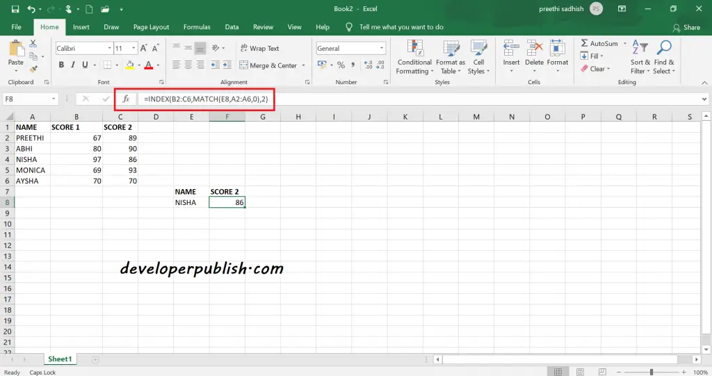
Combination INDEX and MATCH performs as same as VLOOKUP. INDEX returns a value of a cell in a table based on the column and row number whereas MATCH returns the position of a cell.
=INDEX(result_range, MATCH(lookup_value, lookup_range, 0))

