SUMIF Function in Excel
In this post, let’s learn how the SUMIF function works in excel, describe the formula syntax, and how you can use the SUMIF function in an excel spreadsheet.
What is SUMIF Function in Excel?
The SUMIF Function in Excel is used to sum the values in a range when it meets a certain criterion that you specified.
Syntax of SUMIF Function
=SUMIF (range, criteria, [sum-range])
Parameter
- Range– (Required) The range of cells that was evaluated by criteria.
- Criteria– (Required) The criteria are used to determine the cells to be added.
- Sum_range– (Required) The cells to be added together.
Example
=SUMIF (A2:A9,”>50”)
=SUMIF (G6:G10,”>90”)
How to use SUMIF Function in Excel?
The following steps will explain the work of the SUMIF function in an excel spreadsheet:
- First, prepare an excel sheet with the specified details in it, or open an existing excel sheet.
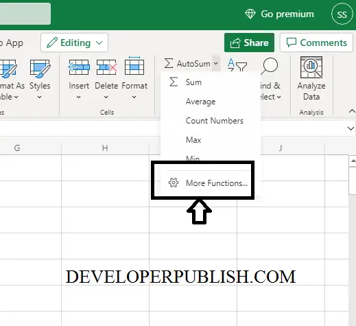
- In the Formulas ribbon, you can see the Auto sum command in it click it a drop-down box will appear, in that choose more functions.
- Home->Auto sum->More Functions
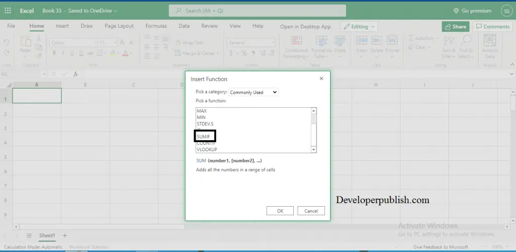
- An insert function dialogue box appears with a drop-down list of various function that choose SUMIF Function in it.
- Insert Function->SUMIF->ok
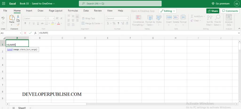
- After that “ =SUMIF( “ appears in the cell where you want to display the result of the SUMIF Function.
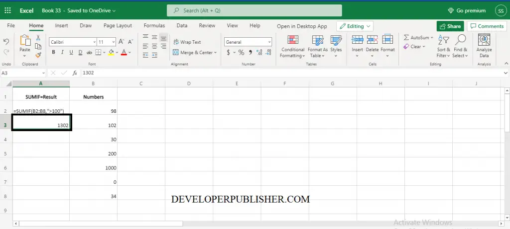
- In cell A3 the result of the SUM of the range between B2:B8 calculates the values that are more than 100. The syntax we have used is “ =SUMIF (B2:B8,”>100″)”
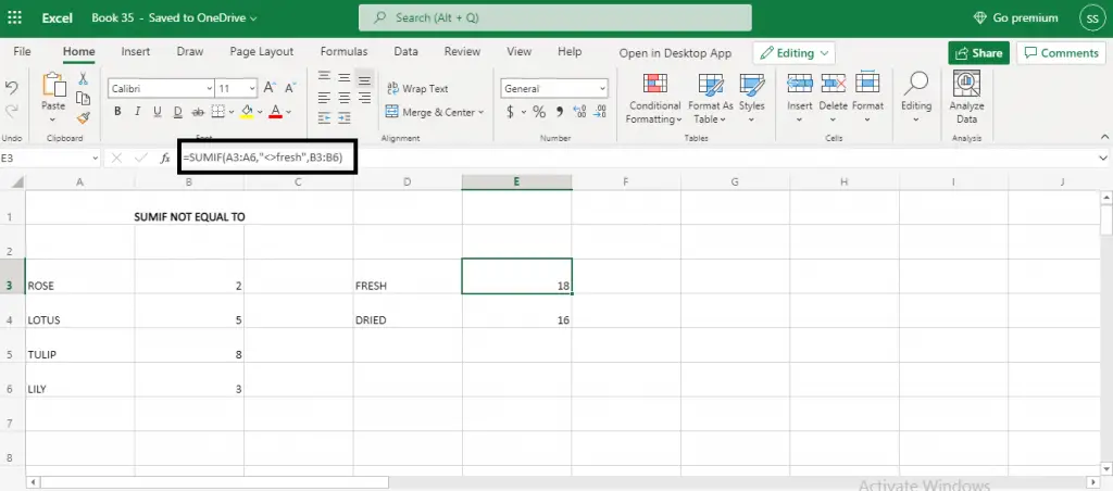
SUMIF NOT EQUAL TO
To perform not equal to criteria use the “<>” operator within double-quotes.
Note:
- The SUMIF Function only supports one condition.



Leave a Review