RANK.AVG Function in Excel
In this article, you will learn about RANK.AVG function, the formula syntax, and usage of the function in Microsoft Excel.
RANK.AVG Function in Excel
The RANK.AVG function in Excel returns the rank of a number against a list of other numeric values. In case of duplicate entries in the array, the RANK.AVG function will assign an average rank to each set of duplicates.
Syntax
=RANK.AVG (number, ref, [order])
Arguments:
- Number – The number whose rank you want to find.
- Ref – An array of, or a reference to, a list of numbers.
- Order – A number specifying how to rank the number
Possible Errors and Usage Notes
- When order is 0 or omitted, the largest value is ranked #1.
- When order is 1, the smallest value is ranked #1.
- Ref with nonnumeric values is ignored by the function.
- It is not necessary to sort the values in the list before using the RANK.AVG function.
How to use the RANK.AVG Function in Excel?
Using this function in a WS is simple; all you need to do is enter the function as a formula of the cell in the formula bar.
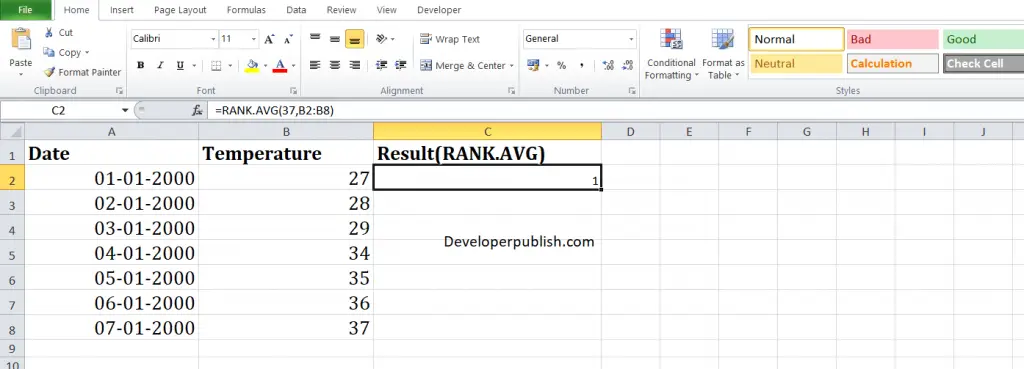
Take a look at the given example

Enter the data in the respective columns and enter the RANK.AVG function formula.
Formula: =RANK.AVG(37, B2:B6,)
Here, A2 refers to the cell name or the cell address. Column A denotes the Date and Column B denotes the ref value. From the given temperature, 37 ranks 1, i.e., it is the highest temperature in the list.


Leave a Review