PERCENTRANK Function in Excel

In this article, you will learn about the PERCENTRANK function, the formula syntax and usage of the function in Microsoft Excel.

PERCENTRANK Function in Excel

The PERCENTRANK function in Excel returns the rank of a value in a data set as a percentage of the data set. This function can be used to evaluate the relative standing of a value within a data set.

The percentile rank is commonly used as the key to interpreting the standing in standardized tests.

Syntax

= PERCENTRANK(array,x,[significance])

Arguments:

• Array    – The array or range of data with numeric values.

• X – The value for which you want to know the rank.

• Significance   – The number of significant digits for the returned percentage value. When omitted, PERCENTRANK uses three digits (0.xxx) in default. (Optional.)

Usage Notes and Possible Errors

• When the array is empty, the PERCENTRANK function returns the #NUM! error value.
• In case of significance being lesser than 1 then, the PERCENTRANK function returns the #NUM! error value.
• And when x does not match one of the values in array, PERCENTRANK interpolates to return the correct percentage rank.

How to use the PERCENTRANK function in Excel?

Using this function in a WS is simple; all you need to do is enter the function as a formula of the cell in the formula bar.

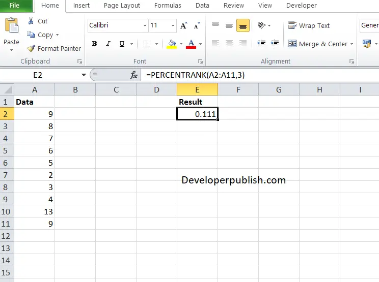
Take a look at the given example

Enter the data in the respective columns and enter the PERCENTRANK formula.

Formula: = =PERCENTRANK(A2:A11,3)

Here, A2 refers to the cell name or the cell address of the array and 3 is the X value (argument). You will get the result in the Result column.

Percent rank of 3 in the range A2:A11. The result is 0.111 because one value in the set is less than 3, and eight are greater than 3. Because 3 is found in the range (cell A6), the number of values less than 3 is divided by the sum of the number of values less than 3 and the number of values greater than 3,  i.e., 1/(1+8)=0.111