MROUND Function in Excel
In this post, you will learn about the MROUND Function, how to use it in your excel spreadsheets.
MROUND Function in Excel
The MROUND function returns a rounded number with a given multiple. The function will round off the numbers either up or down depending on the multiple.
This is one of the rounding off functions in excel like the Ceiling and Floor function.
Syntax
=MROUND(number, significance)
The syntax has two arguments
- number – The number that you want to round up; Required
- significance – The multiple to which you want to round the number; Required
How to use MROUND Function in Excel?
- The function returns the nearest multiple of the given multiple.
- Both the arguments in the syntax can be positive or decimal numbers.
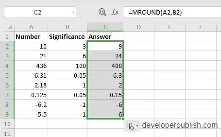
- Note that the number is rounded up according to the multiples and not the number itself Example =CEILING(10, 3) answer is 9 a multiple of 3.
- The function selects the closest multiple to the given number as the answer, whether it is greater or lesser.
- Sometimes when the significance value is 1, the function returns the number unchanged as the answer. This happens when there is no need to round up the number as it satisfies the significance value.
Examples
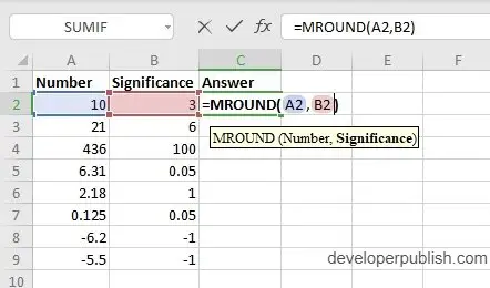
Start with the data. Then in a new cell enter the syntax and highlight the data to insert it in the syntax.
Press enter to display the answer and use the fill handle to apply the function to the rest of the data.
Additional points:
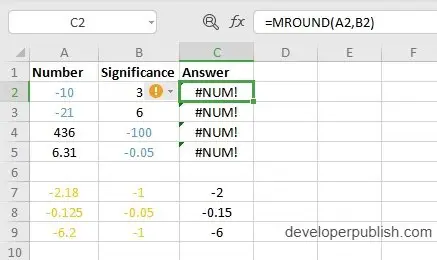
- The function does not work when one of the arguments is a negative number and returns #NUM!.
- When both the arguments are negative the syntax works, and the answer is displayed.
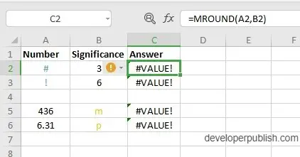
- The syntax returns #VALUE! when the argument is a non – numeric value.


Leave a Review